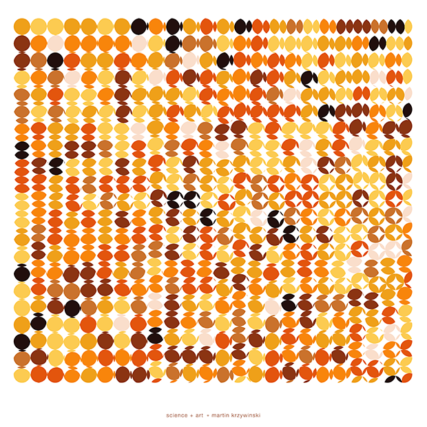
`\pi` Day 2017 Art Posters - Star charts and extinct animals and plants

On March 14th celebrate `\pi` Day. Hug `\pi`—find a way to do it.
For those who favour `\tau=2\pi` will have to postpone celebrations until July 26th. That's what you get for thinking that `\pi` is wrong. I sympathize with this position and have `\tau` day art too!
If you're not into details, you may opt to party on July 22nd, which is `\pi` approximation day (`\pi` ≈ 22/7). It's 20% more accurate that the official `\pi` day!
Finally, if you believe that `\pi = 3`, you should read why `\pi` is not equal to 3.

Caelum non animum mutant qui trans mare currunt.
—Horace
This year: creatures that don't exist, but once did, in the skies.
This year's `\pi` day song is Exploration by Karminsky Experience Inc. Why? Because "you never know what you'll find on an exploration".
create myths and contribute!
Want to contribute to the mythology behind the constellations in the `\pi` in the sky? Many already have a story, but others still need one. Please submit your stories!
If you follow my projects, you know that a big part of the final piece is the story and method behind its creation.
I'm not content to merely show what I have made. By talking about the process, its messiness, failures and successes, I'm hopeful that you'll take away something that will inspire you and help you be more creative and productive in your pursuits.
This year's project has a lot of components and is probably my most ambitious yet. It is a mixture of math and storytelling through patterns and mythologies.
As usual, finding patterns and stories in `\pi` is an ironic pursuit and irony is the best of all wits.
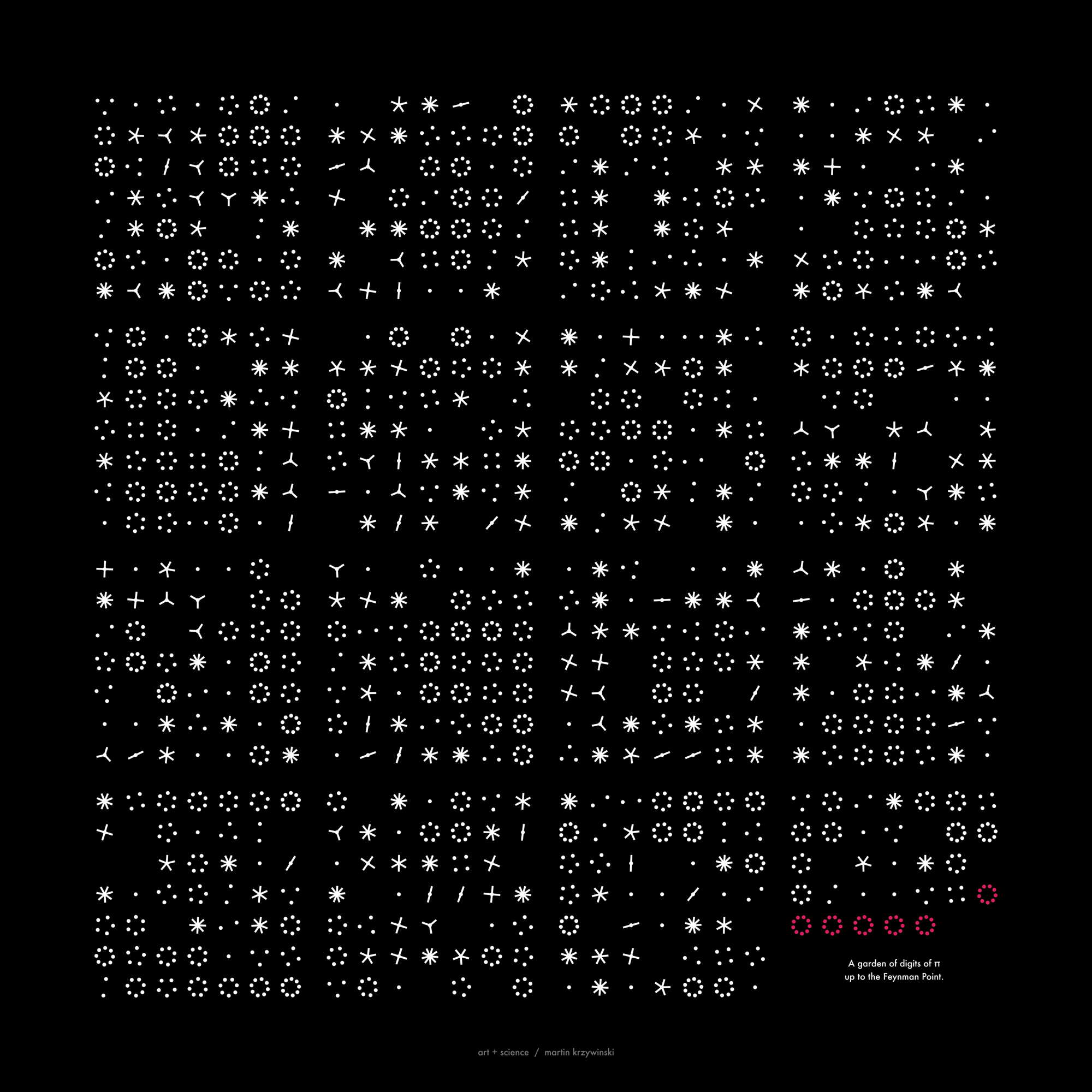
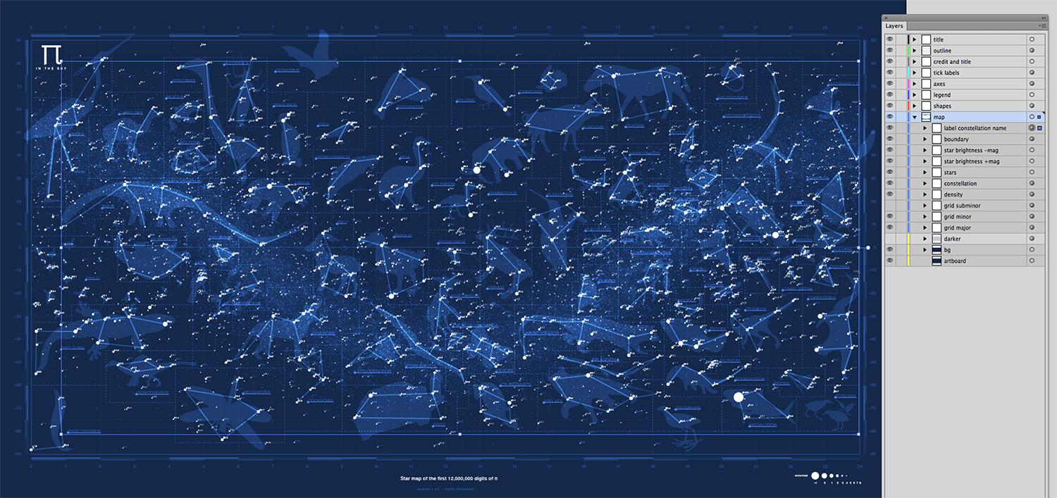
the digits of `\pi` as a star catalogue
The digits of `\pi` are parsed from the start in blocks of 12. The digits in each block are interpreted as the `(x,y,z)` coordinates of the star, with only 3 digits used for the `z` coordinate. The last digit is the absolute magnitude of the star (`M_{abs}`).
       314159265358
       ----++++---+
       x   y   z  Mabs
By parsing the first 12 million digits, you get a million stars. Each star's apparent magnitude, (`M_{app}`) is calculated from its absolute magnitude and its longitude and latitude in the sky is calculated using conversion from Cartesian to spherical coordinates.
#    i digits        name      x      y     z      long     lat         d  Mabs  Mapp
     0 314159265358     a  -1859    926    35  145.339  -38.384  2077.157  3.00 14.59
     1 979323846264     b   4793  -2616   126  -38.404   39.555  5461.884 -1.00 12.69
     2 338327950288     c  -1617  -2205  -472 -110.162  -32.164  2774.797  3.00 15.22
                      ...
999997 420478142596 cexhl   -796   2814  -241   97.939  -14.471  2934.330  1.00 13.34
999998 278256213419 cexhm  -2218    621  -159  156.900  -46.719  2308.776  4.00 15.82
999999 453839371943 cexhn   -462  -1063  -306  -95.924  -26.937  1198.770 -2.00  8.39
The coordinates are centered on zero by subtracting the average coordinate (4999 for `x` and `y` and 499 for `z`) from the sequence of digits.
     3141    5926     535
    -4999.5  4999.5   499.5
     ----    ----     ---
  x -1859  y  926   z  35
apparent brightness
The star's absolute magnitude is in the range -5 (brightest) to 5 (dimmest). The apparent magnitude is given by $$ M_{app} = M_{abs} + 5 \left( \log_{10} d - 1 \right) $$
So for the first star, whose distance from the origin (the location of the observer planet), $$ M_{app} = 3 + 5 \left ( log_{10} 2077.157 - 1 \right) = 3 + 5 \times 2.31 = 14.59 $$
For each difference in one apparent magnitude, the change in brightness is a factor of `100^{1/5} = 2.5`.
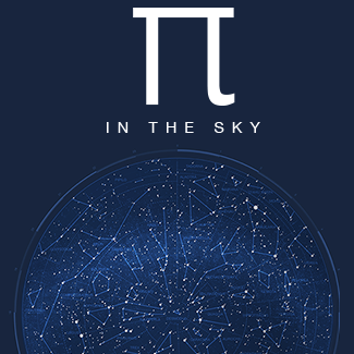
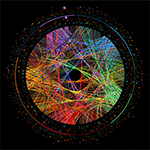
exploring projections
The stars' position in the universe `(x,y,z)` are projected onto the unit sphere to calculate their longitude `-180 .. 180` and latitude `-90 .. 90` coordinates.
Once this is done the next step is to figure out how to project the unit sphere onto the page.

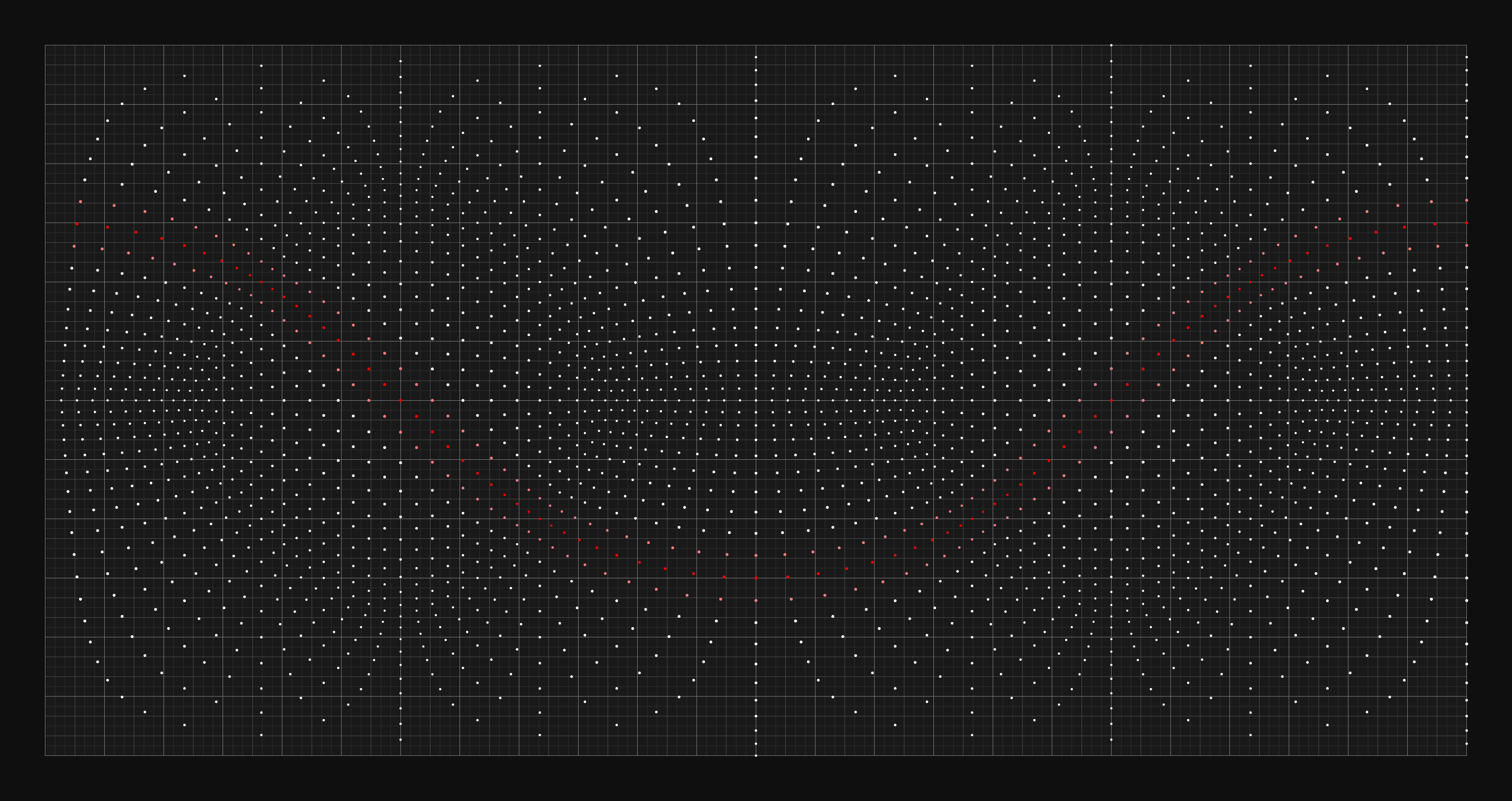
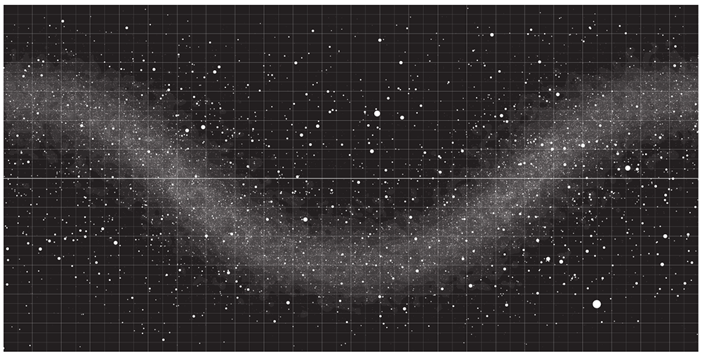
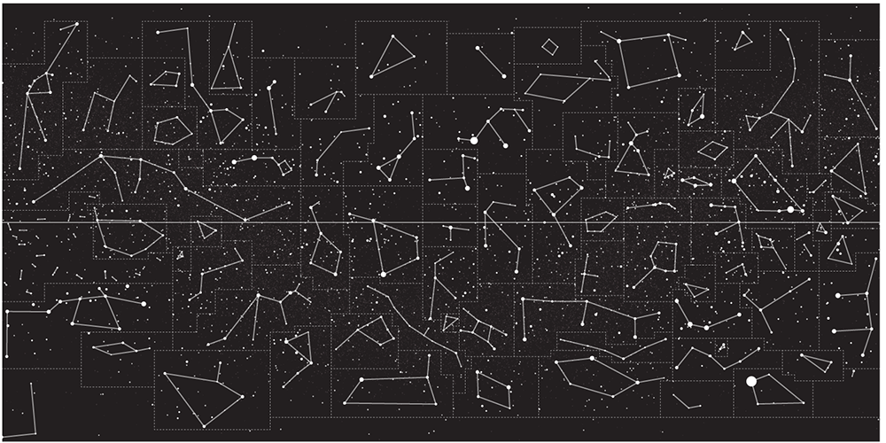
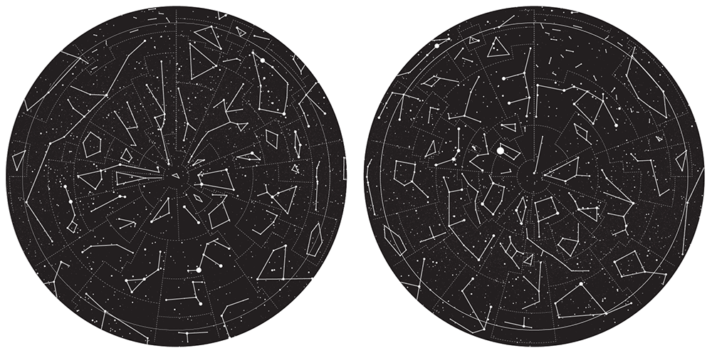
There is a huge number of topographical projections to choose from. In star charts, some common ones are plate Carrée and azimuthal equidistant projections.
The Carrée simply maps lines of latitude and longitude to equally spaced lines. The azimuthal equidistant projection is more complicated and has the property that all points on the map are at proportionately correct distances from the center point. The flag of the United Nations uses this kind of projection.
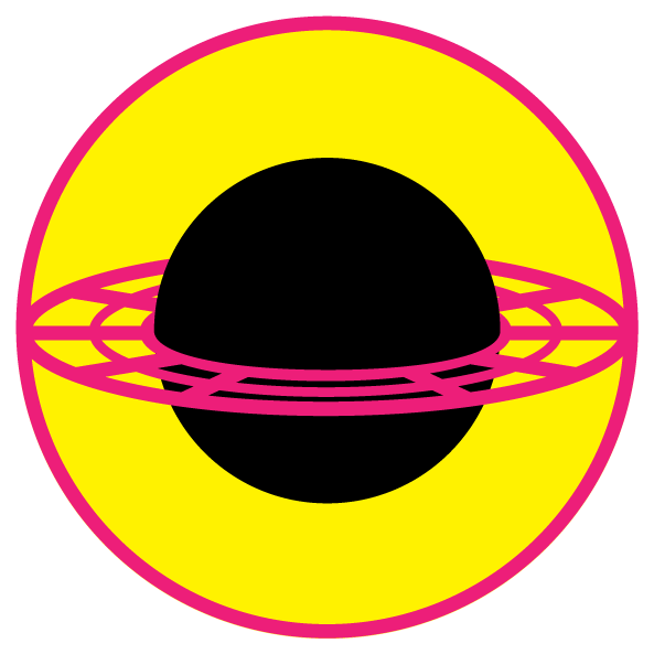
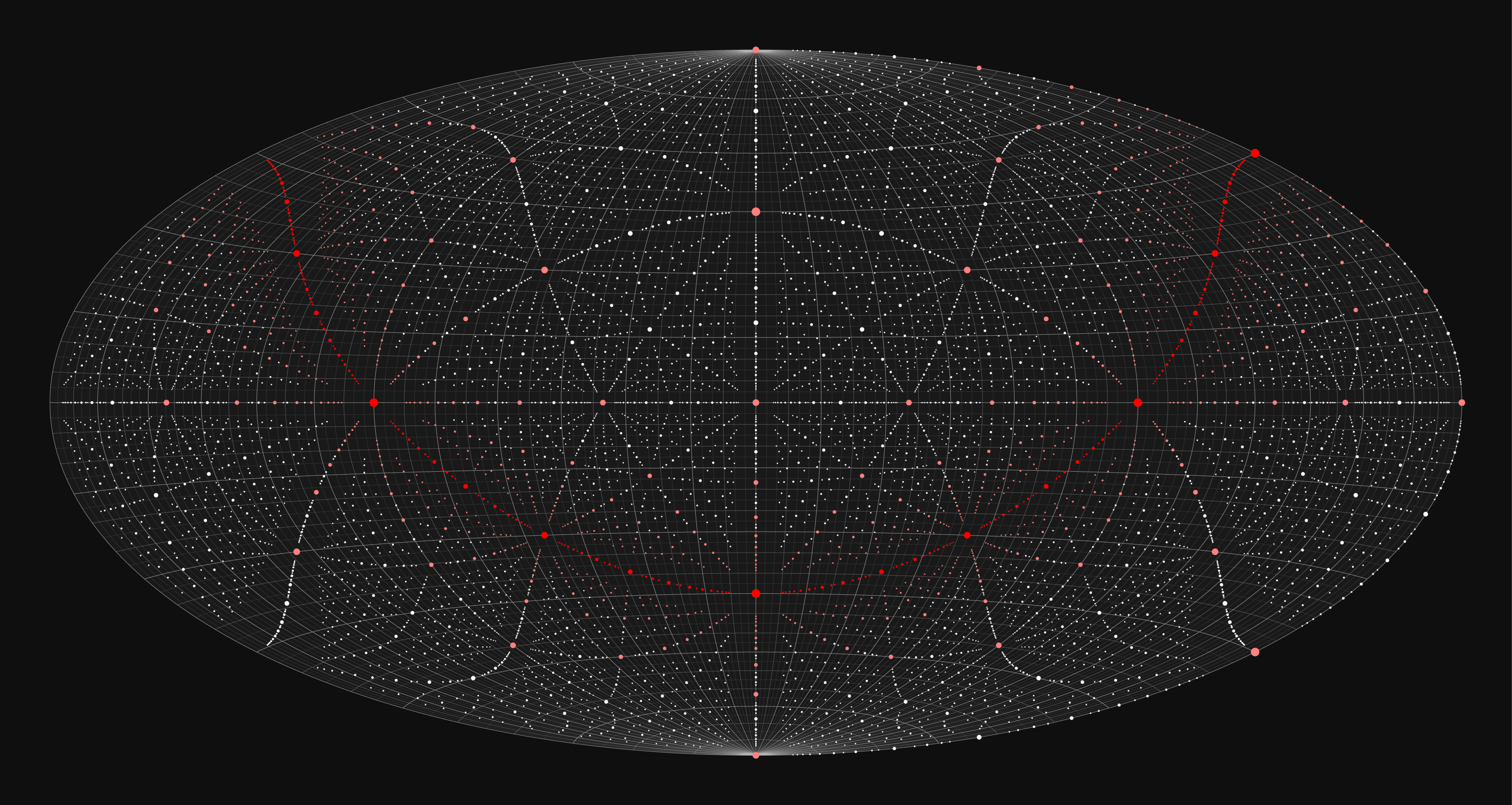
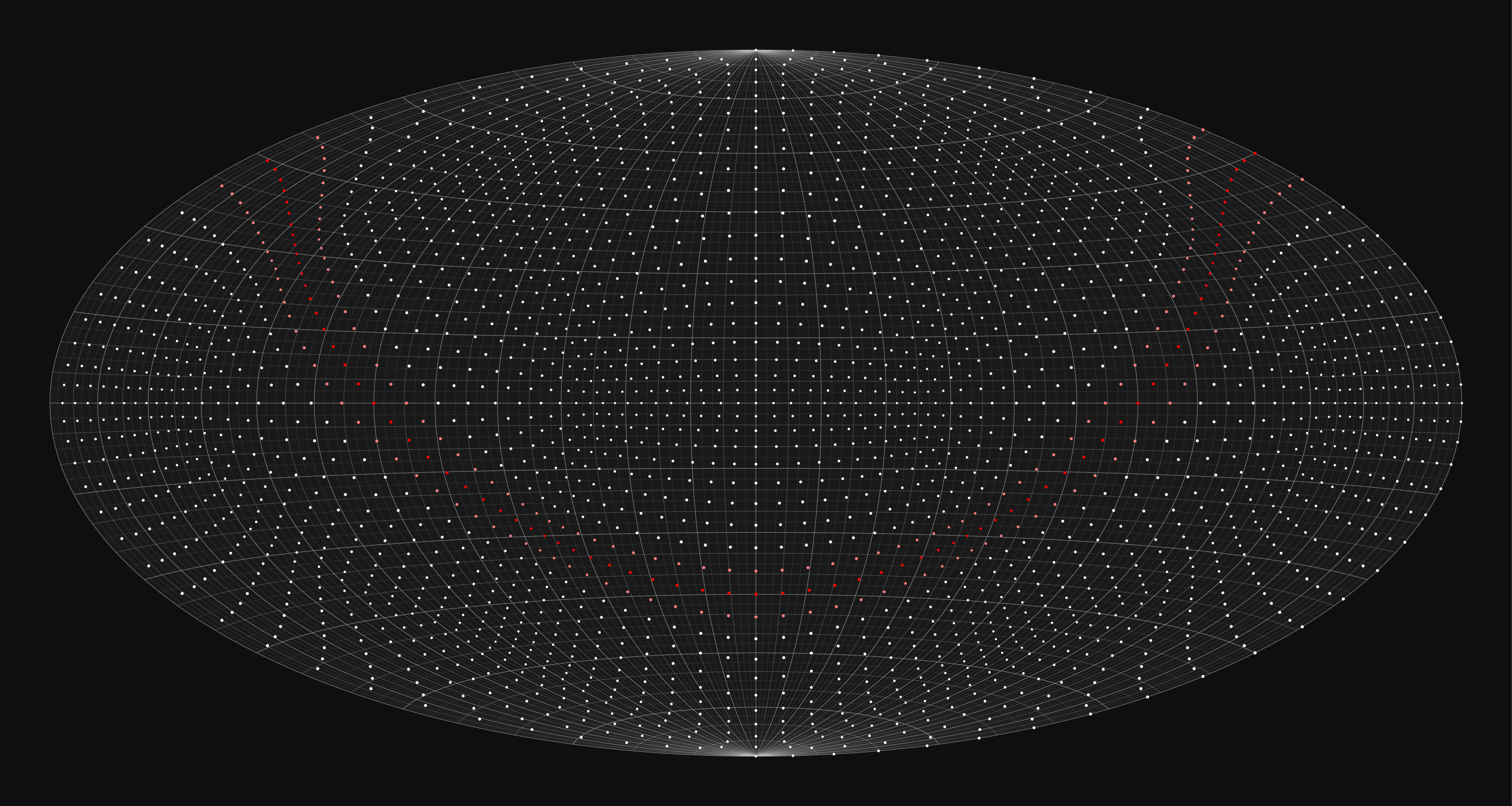
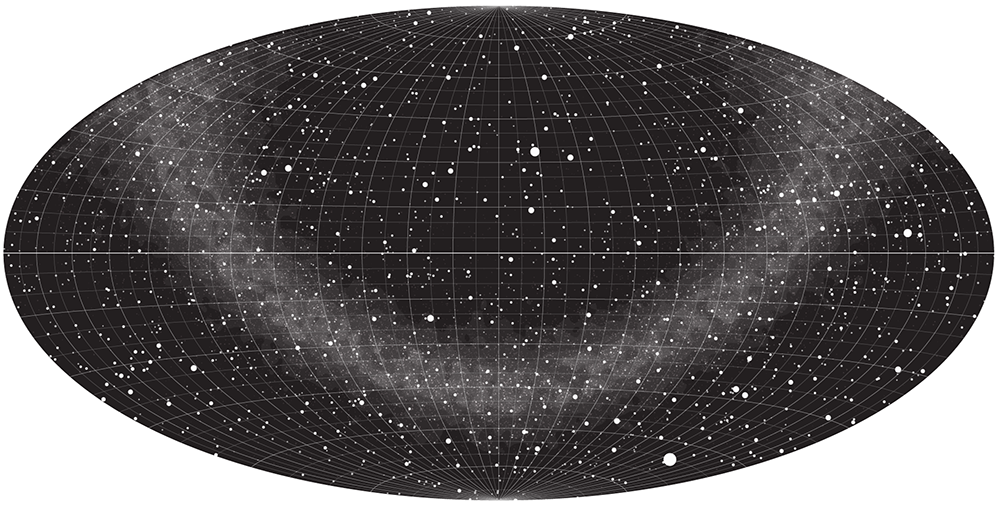
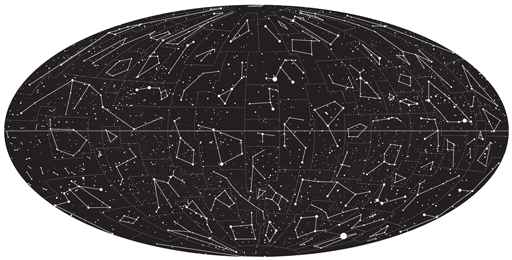
I also wanted to explore the Mollweide projection because this is the one used in the famous background microwave background radiation image. This projection has some artefacts around the edges so instead I used the very similar Hammer/Aitoff projection, which has less distortion at the outer meridians.
The discussion of whether to use Mollweide or Hammer is a hot topic of debate at xkcd. Maybe one day I'll make a Mollweide map too.
At this point it would be criminal of me not to acknowledge Craig DeForest's PDL::Transform::Cartography module. I had a few questions about syntax and he wrote back to me within a few hours of my query.
To be honest, I haven’t used t_vertical since I got t_perspective online (some 12 or so years ago). I'll have a look at it tonight and try to get you a useful answer. Stand by a couple of hours—it’s putting-down-kids-to-bed time.
—Craig DeForest
That is the most awesome support I have ever received!
a cube of stars
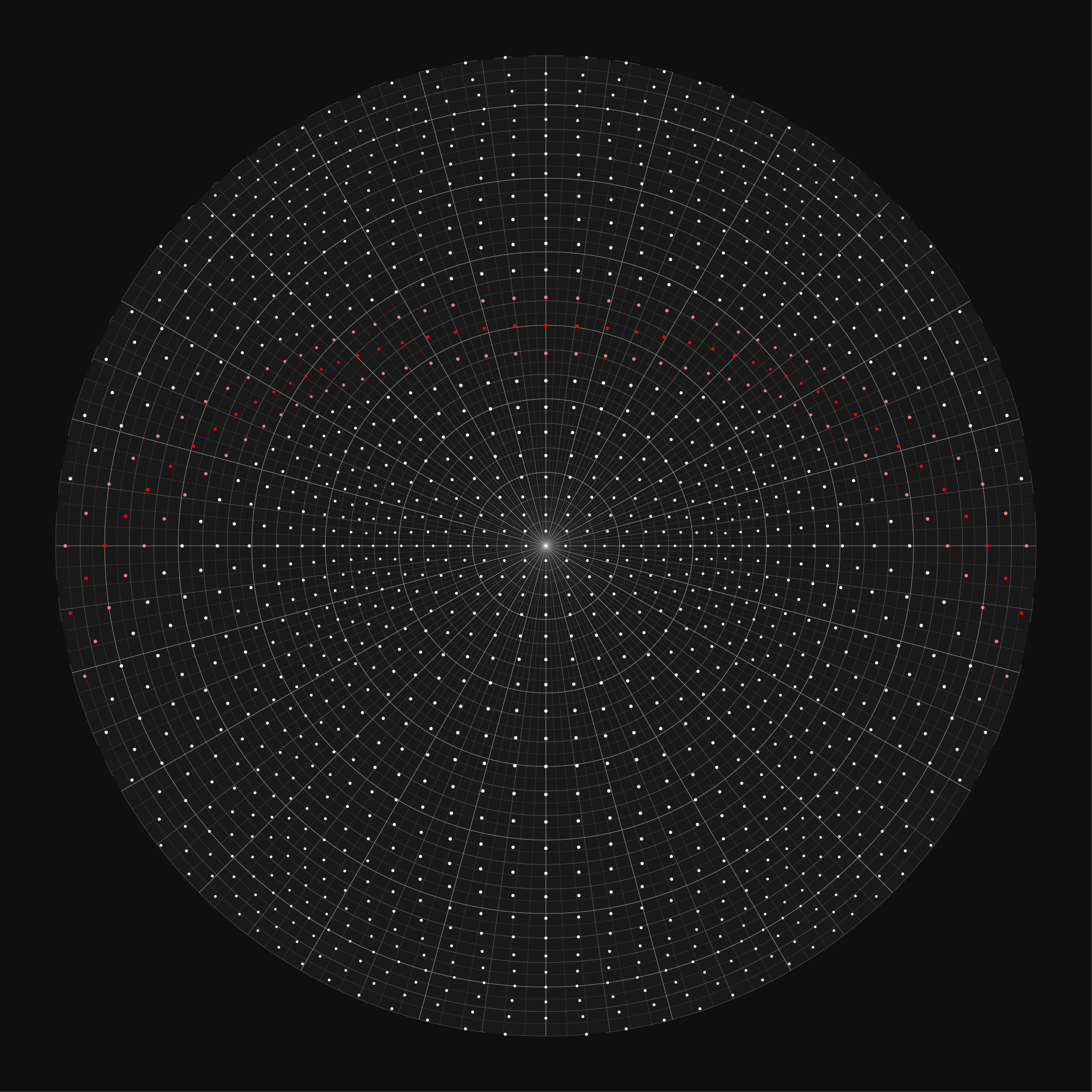
To illustrate how an arrangement of stars looks in each projection, let's start with a cube of stars.
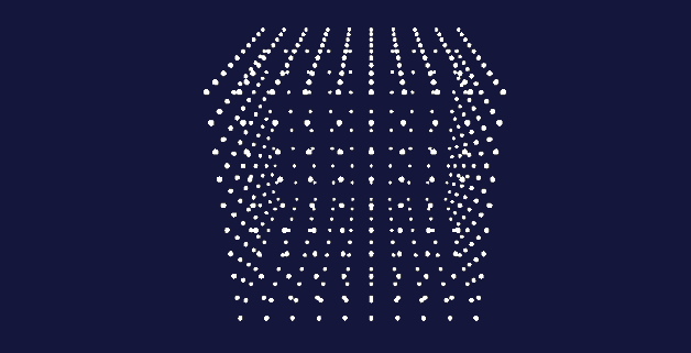
For this, I created a catalog of stars that fill the cube centered on (0,0,0) and having an edge length of 10,000. This size of cube represents the limits of the coordintaes in the catalog based on the digits of `\pi`. I arbitrarily set the absolute magnitude of each star to -8 and use the same star size encoding on here as in the final chart.
Stars close to the "galactic plane" (`z` coordinate close to zero) are tinted red. As for the final charts, the observer planet is rotated so that this plane approximates how the Milky Way looks in actual charts.
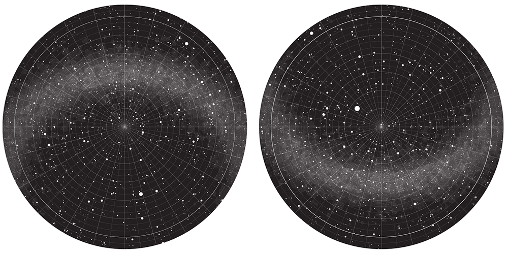
In the azimuthal projection, I decided to show a little bit of the opposite hemisphere. The north hemisphere map range is `[-10,90]` and the south hemisphere range is `[-90,10]`. This provides some continuity around the edges. The bright white circle near the edge of the hemispheres represents the celestial equator.
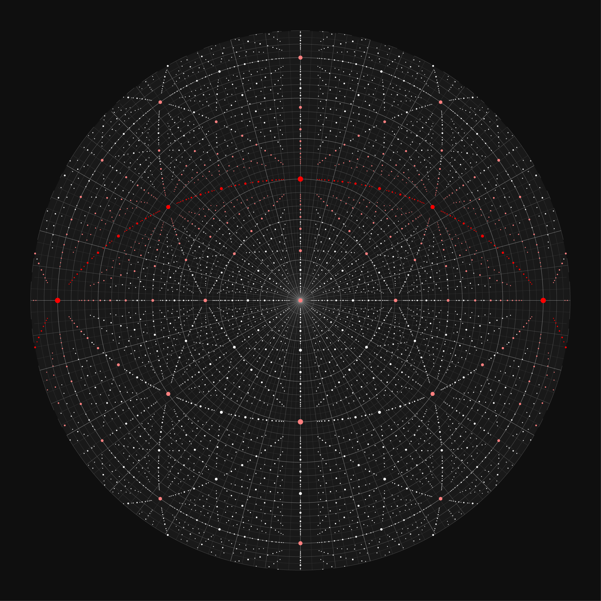
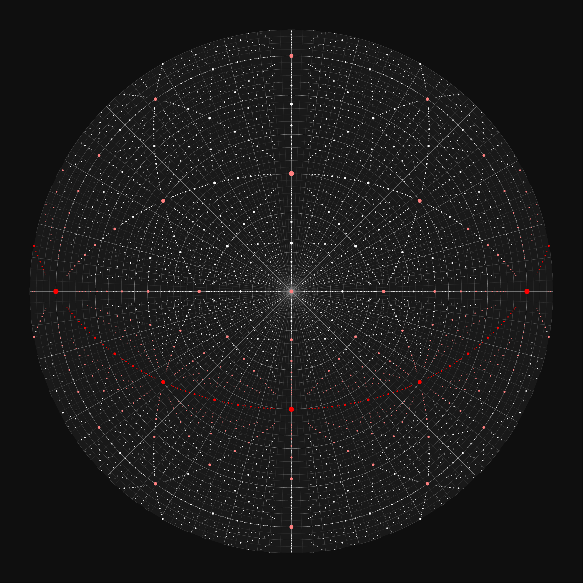
It's interesting to see where the stars that fall on the faces of the cube wind up on the chart. These represent the furthest reaches of this synthetic universe.

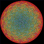
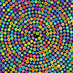
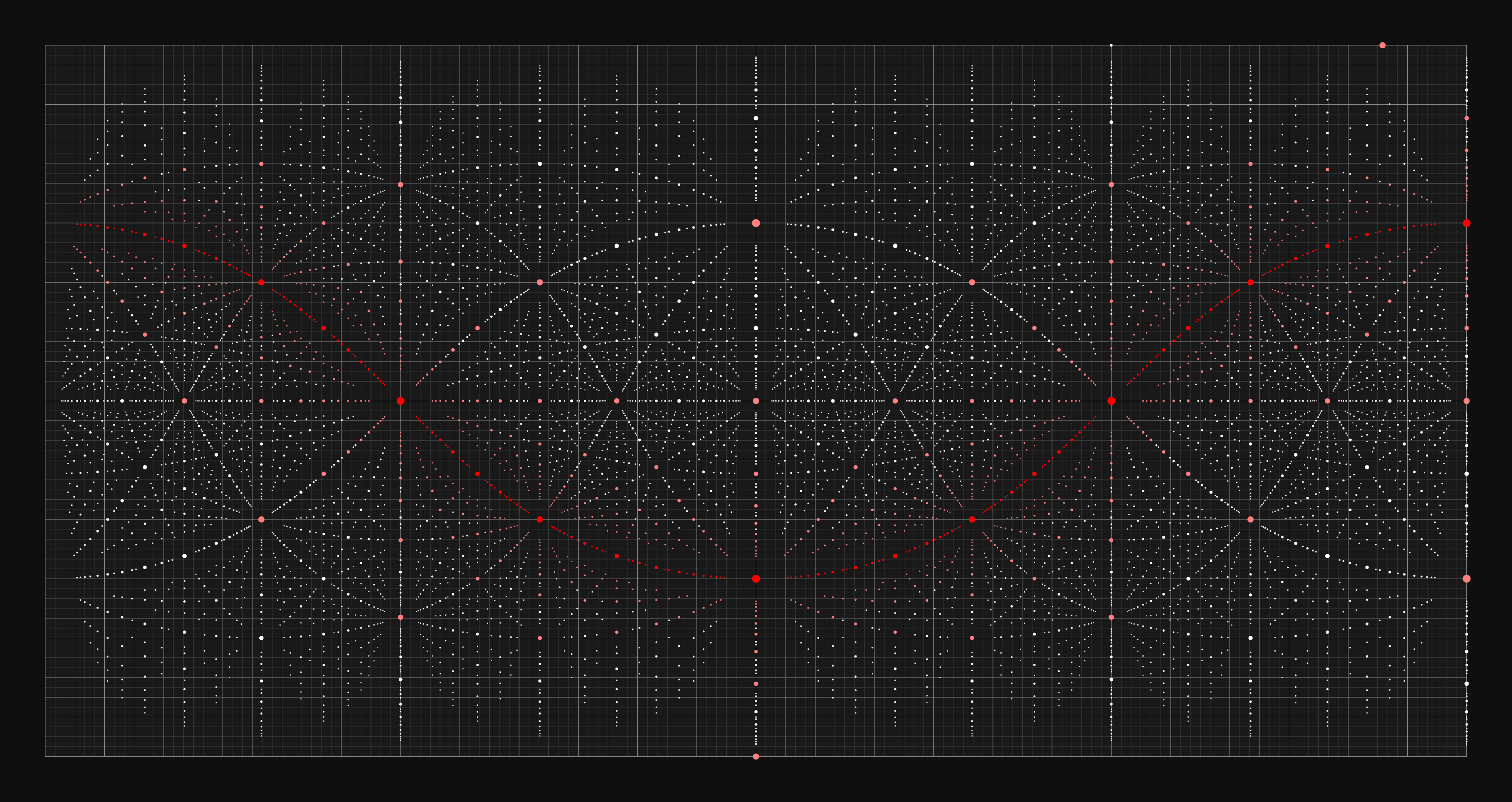
what does randomness look like?
Let's look at what a random distribution of stars looks like on the charts. The final `\pi` star charts draw 40,000 stars from the first 12,000,000 digits, so let's create a catalog of 40,000 stars in which the location of the star is uniformly randomly distributed within a cube. The stars will have random absolute magnitude in the range -5 to 5.
This is roughly what we can expect from `\pi`, since the number is likely normal.
These images are best viewed when zoomed in—go ahead, click on them.
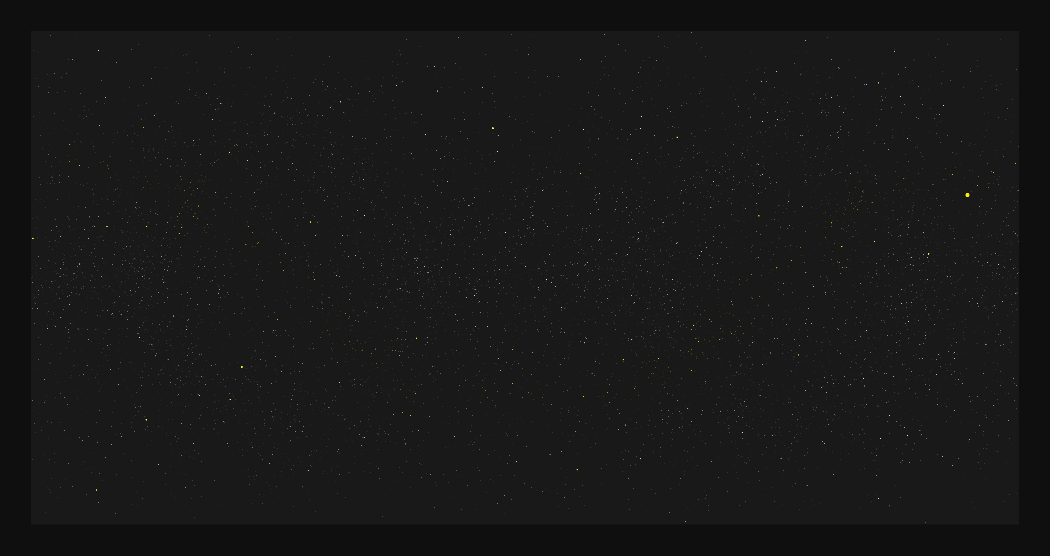
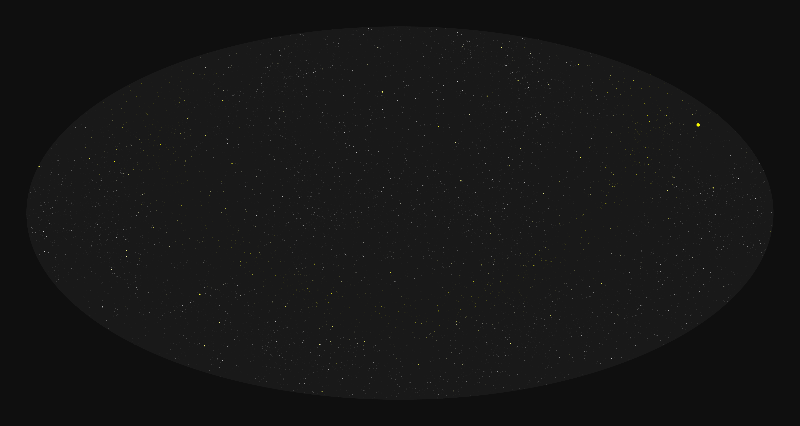
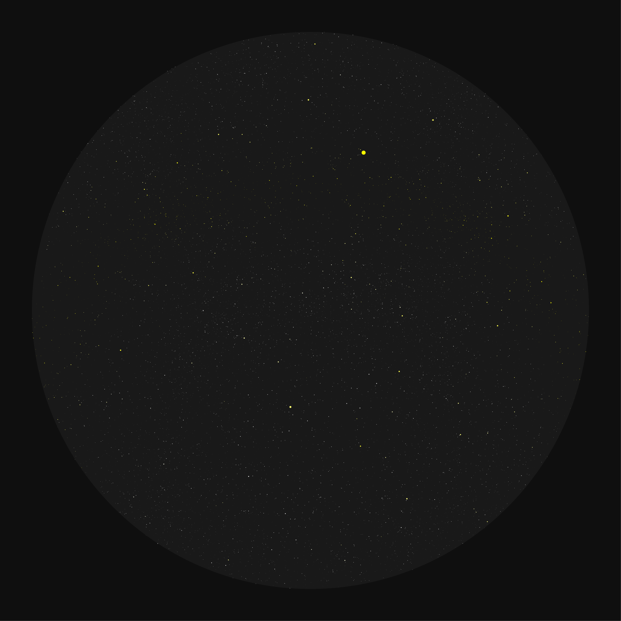
If we fill a cube (or a sphere) with digits in this way, we're not going to wind up with anything particularly intersting. We'll see randomness—and that's ok!— but I wanted the chart to more resemble an actual sky chart.
Let's add some anisotropy!
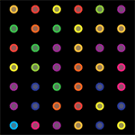
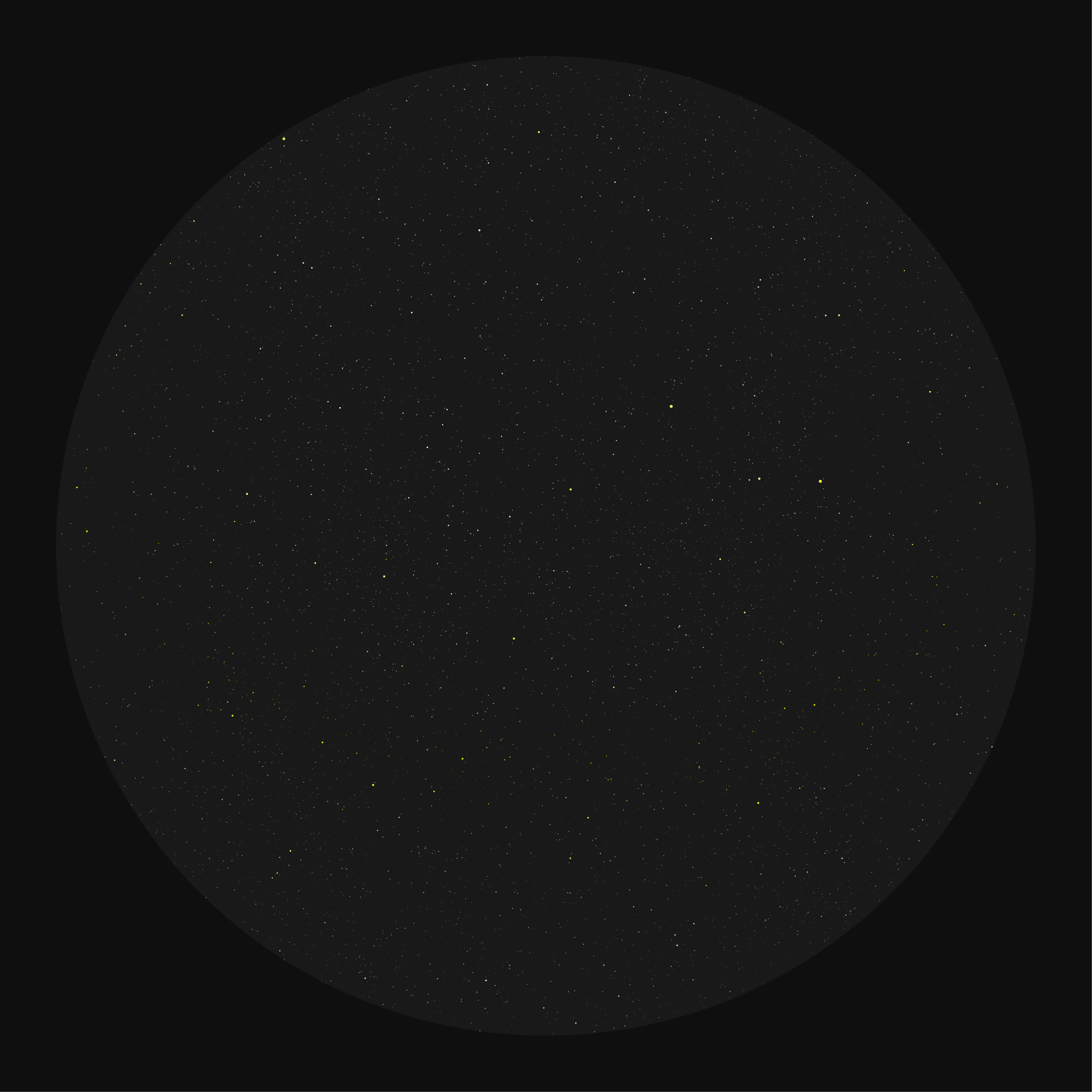
creating anisotropy
If you were paying particular attention, you may be wondering why the `z` coordinate was determined by only 3 digits.
Because the digits of `\pi` are without pattern (the digit is thought to be normal, meaning that in any subsequence all the digits have the same chance of appearing, a universe created from its digits is going to be isotropic. In other words, it will look the same in all directions—uniformly random!
I knew I wanted the chart to have a look similar to the charts of our sky—with a bright band of stars, which in our sky represent the stars within the plane of the Milky Way.
By using only 3 digits for the `z` coordinate and 4 digits for `x` and `y`, the universe of stars doesn't fill a cube but a flat 3-d rectangle. It's 10 times thinner than it is wide.
By rotating the observer planet, I was able to match the location of the band in my star chart to roughly that of the Milky Way in standard charts.
Although the charts only show 40,000 stars (up to apparent magnitude of about –8), more are used to determine the glow of the bands shown in the charts above. To do this, I divided the chart into a 240 × 160 grid and counted the number of stars in each grid. Then, the counts were smoothed and 25, 50, 75, 90, 95 and 99 percentile contours were calculated to provide layering in the bands.
constellations
I knew from the beginning that the constellations would play a big role in the chart. If we think of `\pi` as a star catalogue, then it makes sense that it doesn't include any information about constellations, since these change with time and position of the observer.
It is up to us (me) to look up and figure out patterns.
But how to name the constellations? This plagued me for a long time.
Famous mathematicians? No, that's exactly what people would expect.
Mathematical formulae that use `\pi`? Fun and each equation has a story, but I didn't want it to get too arcane.
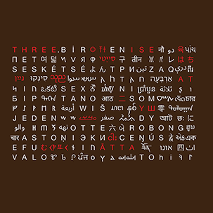
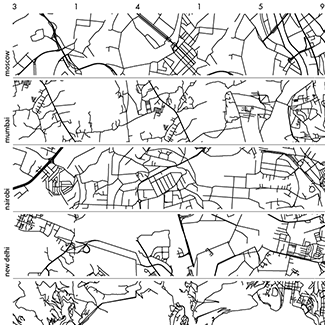
Projecting names of places on the Earth on the corresponding part of the sky? This initially sounded like a great way to sample strange and interesting names and set up a double projection on the chart—up from the Earth and down from space.
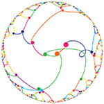
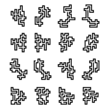
Below is an early attempt at drawing some kind of patterns in the sky. The shapes weren't motivated by anything in particular.
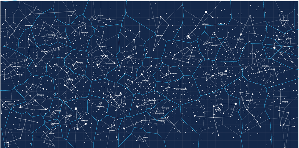
I wasn't very happy with just drawing random shapes. I also wasn't very happy with the boundaries of the constellations being created from a mindless tesselation. Real constellation boundaries usually fall parallel to longitude and latitude lines and the tesselated boundaries didn't look anything like that.
Then I had a better idea.
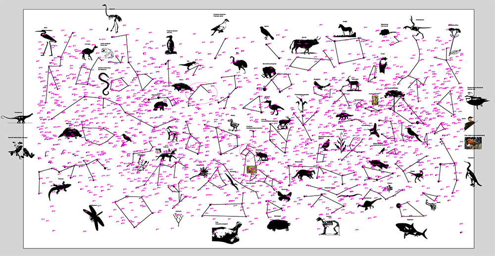
populating the sky with critters and veggies
I was going to populate the sky with extinct plants and animals.
I wanted the constellations to be an homage to the wonderful way Nature has a way of arranging molecules into living things, in part a poetic statement about the passage of time and life and in part a source of mythology for the chart.
After all, most of us have personalities. It's reasonable to expect that these animals did too—behaviour is the fun part of life.
I was quickly met with giant lists of extinct species. Independently, I discovered that if you add "list" to any Google search query you'll be kidnapped by clickbait and listicles, of the worst kind: "10 reasons why your cat wants you extinct". Just kidding. Or not.
It took me a good week to work through the lists and collect animals that seemed to have interesting stories. There are 88 constellations in our sky and I managed to create a new set of 80. Finding patterns in randomly placed dots on the screen is partly fun and slightly frustrating. Oh, look, that definitely looks like a Dodo. Wait. Now this here definitely looks like a Dodo. I was seeing Dodos everywhere.
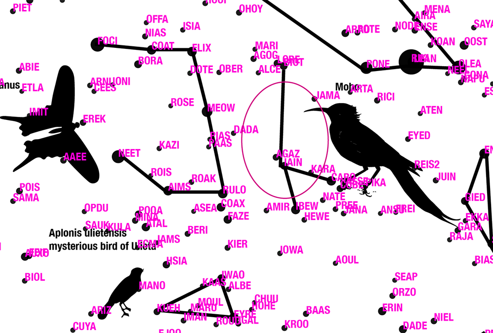
Once I had some clipart of the species on the artboard, I started looking for patterns. I labeled stars with short readable words from the dictionary (e.g. 4-5 letters long with 2 vowels). In the catalogue they're mindlessly coded from a to cexhn, which are hard to type. Then, I went to work defining graph edges that would be the constellations.
Once I had them drawn, I translated the readable words into the original star labels to have a constellation file like this:
# a winding constellation
rodhocetus:
bbiam kefp bxisk bvzam camyi xzhs

# several edges
pterodactyl:
soew brxrr bjass bpftr baelv brnhi kxfu jjco
baelv bkpew

# the trailing . indicates a closed shape
traversia:
puib fywb fcnw .
After finding some constellations, I was showing my work to Jake Lever, a colleague who is often an excellent inspiration for ideas. We've co-authored some Points of Significance columns, so I know Jake is really sharp.
I was complaining to Jake that I was having trouble with the Polygon clipper library, which sometimes wasn't merging polygons that shared an edge. I wanted to automate as much of the process as possible, I said, and didn't want to draw the boundaries of the constellations by hand.
As soon as I said this, I thought... but I really should do them properly. I was using automation as a way to not spend making the sky charts even more excellent.
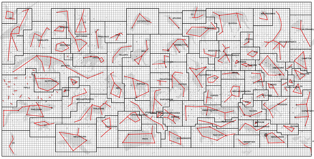
The boundaries actually didn't take that long to draw. Perhaps 20 minutes of making unions of boxes in Illustrator. But then I had to get the position of those shapes back into my star chart drawing code so that I could use it for other projections. Up to now, I was doing all the work in the plate carrée projection. This meant that I had to go back to the code and make everything less of a complete kludge. Damn it, I'm a prototyper not a software developer!
In the end, I think this step was not only worth it but necessary and made the chart appear more authentic.
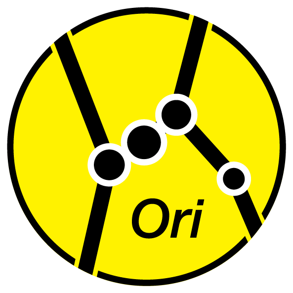
adding star labels
Most stars don't have memorable names. Not everyone can be a Betelgeuse or Rigel.
To help identify stars, they are labeled by their constellation (e.g. Orion) and their relative brightness within that constellation compared to other stars. Because Betelgeuse is the brightest it is first and given the name α Orionis. Rigel is second brightest, so it is β Orionis. The third brightest star is γ, and so on.
I added a layer of labels. All stars brighter than apparent magnitude 4.5 have labels along with any stars that are used to draw the shape of the constellation shape, if they're dimmer. The labels range from α to ω.

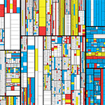
putting it together
The individual components of the chart were generated in SVG, which was then imported into Illustrator. Below is a look at the layer organization.
I am grateful to the music of Hooverphonic and Chicane to sustain long hours of coding, finding shapes of animals and imagining their stories. And, as always, Galileo coffee which sustains our entire genome center.
There's not just truth in coffee, but life.
Nasa to send our human genome discs to the Moon
We'd like to say a ‘cosmic hello’: mathematics, culture, palaeontology, art and science, and ... human genomes.


Comparing classifier performance with baselines
All animals are equal, but some animals are more equal than others. —George Orwell
This month, we will illustrate the importance of establishing a baseline performance level.
Baselines are typically generated independently for each dataset using very simple models. Their role is to set the minimum level of acceptable performance and help with comparing relative improvements in performance of other models.

Unfortunately, baselines are often overlooked and, in the presence of a class imbalance5, must be established with care.
Megahed, F.M, Chen, Y-J., Jones-Farmer, A., Rigdon, S.E., Krzywinski, M. & Altman, N. (2024) Points of significance: Comparing classifier performance with baselines. Nat. Methods 20.
Happy 2024 π Day—
sunflowers ho!
Celebrate π Day (March 14th) and dig into the digit garden. Let's grow something.

How Analyzing Cosmic Nothing Might Explain Everything
Huge empty areas of the universe called voids could help solve the greatest mysteries in the cosmos.
My graphic accompanying How Analyzing Cosmic Nothing Might Explain Everything in the January 2024 issue of Scientific American depicts the entire Universe in a two-page spread — full of nothing.

The graphic uses the latest data from SDSS 12 and is an update to my Superclusters and Voids poster.
Michael Lemonick (editor) explains on the graphic:
“Regions of relatively empty space called cosmic voids are everywhere in the universe, and scientists believe studying their size, shape and spread across the cosmos could help them understand dark matter, dark energy and other big mysteries.
To use voids in this way, astronomers must map these regions in detail—a project that is just beginning.
Shown here are voids discovered by the Sloan Digital Sky Survey (SDSS), along with a selection of 16 previously named voids. Scientists expect voids to be evenly distributed throughout space—the lack of voids in some regions on the globe simply reflects SDSS’s sky coverage.”
voids
Sofia Contarini, Alice Pisani, Nico Hamaus, Federico Marulli Lauro Moscardini & Marco Baldi (2023) Cosmological Constraints from the BOSS DR12 Void Size Function Astrophysical Journal 953:46.
Nico Hamaus, Alice Pisani, Jin-Ah Choi, Guilhem Lavaux, Benjamin D. Wandelt & Jochen Weller (2020) Journal of Cosmology and Astroparticle Physics 2020:023.
Sloan Digital Sky Survey Data Release 12
Alan MacRobert (Sky & Telescope), Paulina Rowicka/Martin Krzywinski (revisions & Microscopium)
Hoffleit & Warren Jr. (1991) The Bright Star Catalog, 5th Revised Edition (Preliminary Version).
H0 = 67.4 km/(Mpc·s), Ωm = 0.315, Ωv = 0.685. Planck collaboration Planck 2018 results. VI. Cosmological parameters (2018).
constellation figures
stars
cosmology
Error in predictor variables
It is the mark of an educated mind to rest satisfied with the degree of precision that the nature of the subject admits and not to seek exactness where only an approximation is possible. —Aristotle
In regression, the predictors are (typically) assumed to have known values that are measured without error.
Practically, however, predictors are often measured with error. This has a profound (but predictable) effect on the estimates of relationships among variables – the so-called “error in variables” problem.

Error in measuring the predictors is often ignored. In this column, we discuss when ignoring this error is harmless and when it can lead to large bias that can leads us to miss important effects.
Altman, N. & Krzywinski, M. (2024) Points of significance: Error in predictor variables. Nat. Methods 20.
Background reading
Altman, N. & Krzywinski, M. (2015) Points of significance: Simple linear regression. Nat. Methods 12:999–1000.
Lever, J., Krzywinski, M. & Altman, N. (2016) Points of significance: Logistic regression. Nat. Methods 13:541–542 (2016).
Das, K., Krzywinski, M. & Altman, N. (2019) Points of significance: Quantile regression. Nat. Methods 16:451–452.
Convolutional neural networks
Nature uses only the longest threads to weave her patterns, so that each small piece of her fabric reveals the organization of the entire tapestry. – Richard Feynman
Following up on our Neural network primer column, this month we explore a different kind of network architecture: a convolutional network.
The convolutional network replaces the hidden layer of a fully connected network (FCN) with one or more filters (a kind of neuron that looks at the input within a narrow window).
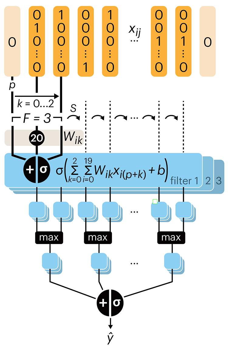
Even through convolutional networks have far fewer neurons that an FCN, they can perform substantially better for certain kinds of problems, such as sequence motif detection.
Derry, A., Krzywinski, M & Altman, N. (2023) Points of significance: Convolutional neural networks. Nature Methods 20:1269–1270.
Background reading
Derry, A., Krzywinski, M. & Altman, N. (2023) Points of significance: Neural network primer. Nature Methods 20:165–167.
Lever, J., Krzywinski, M. & Altman, N. (2016) Points of significance: Logistic regression. Nature Methods 13:541–542.