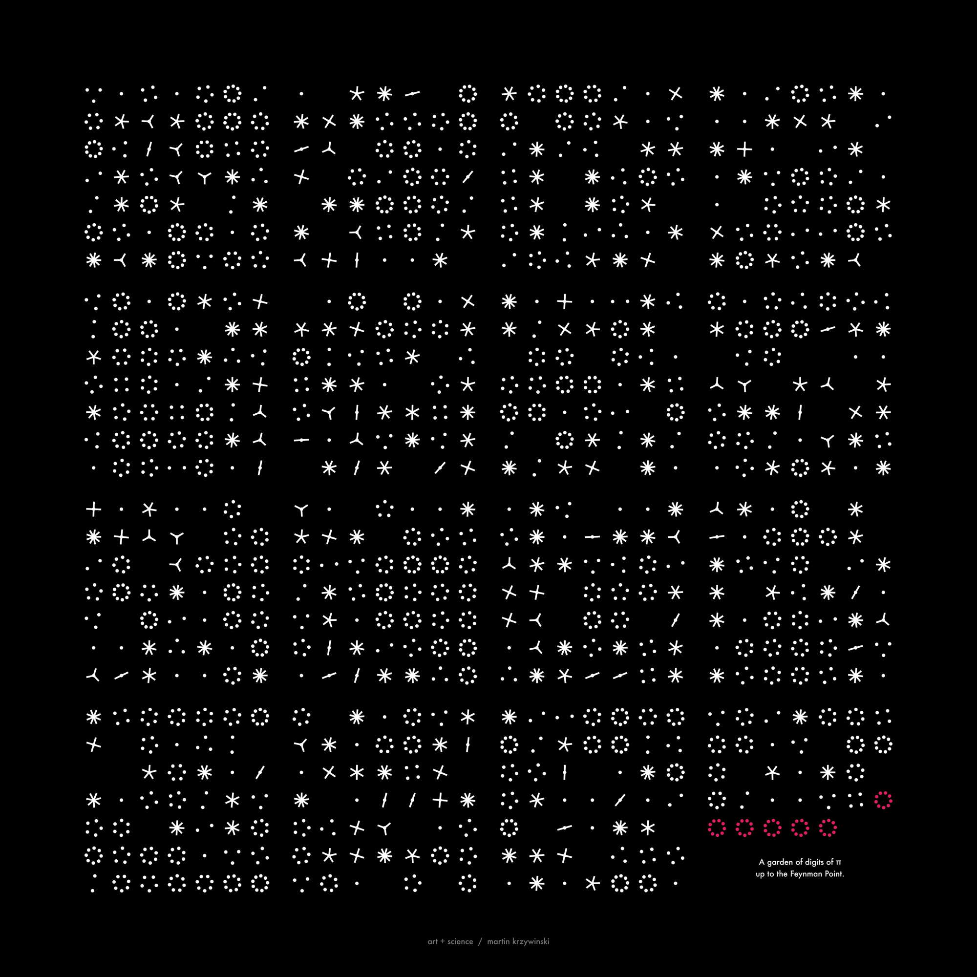
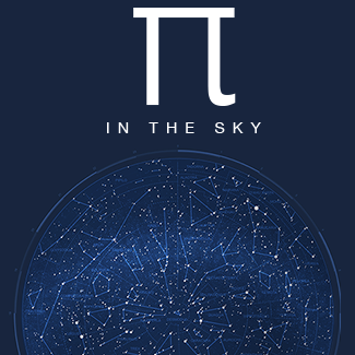
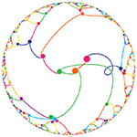
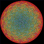
`\pi` Day 2017 Art Posters - Star charts and extinct animals and plants


On March 14th celebrate `\pi` Day. Hug `\pi`—find a way to do it.
For those who favour `\tau=2\pi` will have to postpone celebrations until July 26th. That's what you get for thinking that `\pi` is wrong. I sympathize with this position and have `\tau` day art too!
If you're not into details, you may opt to party on July 22nd, which is `\pi` approximation day (`\pi` ≈ 22/7). It's 20% more accurate that the official `\pi` day!
Finally, if you believe that `\pi = 3`, you should read why `\pi` is not equal to 3.

Caelum non animum mutant qui trans mare currunt.
—Horace
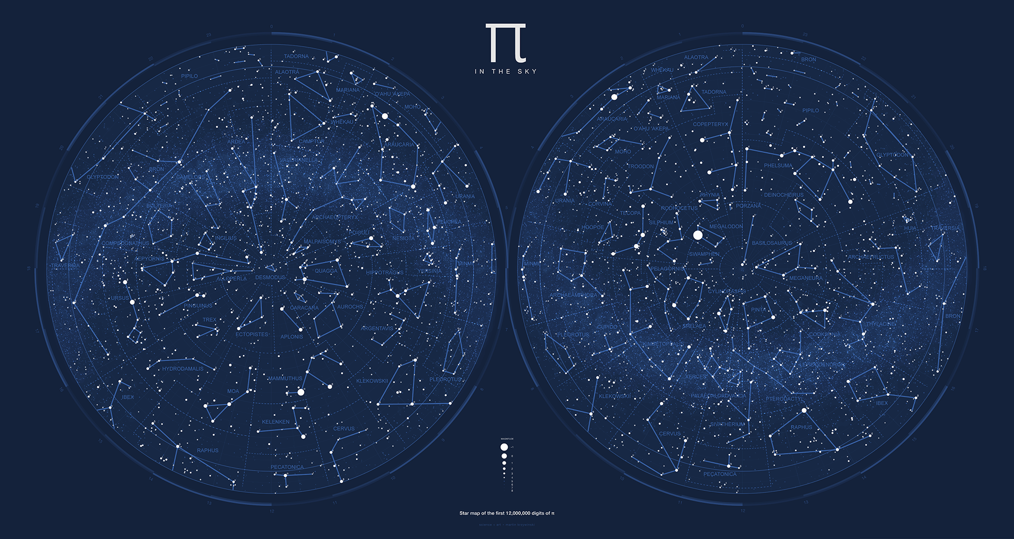
This year: creatures that don't exist, but once did, in the skies.
This year's `\pi` day song is Exploration by Karminsky Experience Inc. Why? Because "you never know what you'll find on an exploration".


create myths and contribute!
Want to contribute to the mythology behind the constellations in the `\pi` in the sky? Many already have a story, but others still need one. Please submit your stories!
Here I make available all the files you need to reconstruct the chart. All files are plain text and designed to be easily parsable.
 buy artwork
For the simplest chart, you'll need the star catalogue which already provides the longitude and latitude coordinates for each star. It'll be up to you to choose and calculate a projection.
You can then layer constellations, which are defined by a list of edges. If you like, you can draw boundaries around each constellation, which are also provided.
Star-to-constellation mapping is also given, which allows you to create labels for the stars within each constellation based on relative brightness.
Finally, you can get the species details for each constellation, including the Latin name of the species, Wikipedia URL and (for many) the mythology of the constellation.
star catalogue
The star catalog generated from the first 12 million digits of `\pi`.
DOWNLOAD

#   idx       digits   name      x      y      z     long      lat      dist  mabs  mapp
      0 314159265358      a  -1859    926     35  145.339   38.384  2077.157  3.00 14.59
      1 979323846264      b   4793  -2616    126  -38.404  -39.555  5461.884 -1.00 12.69
      2 338327950288      c  -1617  -2205   -472 -110.162   32.164  2774.797  3.00 15.22
      3 419716939937      d   -803  -3307    493 -105.489    3.655  3438.620  2.00 14.68
...
 999996 601538500580  cexhk   1015  -1150   -442  -48.144  -14.704  1596.273 -5.00  6.02
 999997 420478142596  cexhl   -796   2814   -241   97.939   14.471  2934.330  1.00 13.34
 999998 278256213419  cexhm  -2218    621   -159  156.900   46.719  2308.776  4.00 15.82
 999999 453839371943  cexhn   -462  -1063   -306  -95.924   26.937  1198.770 -2.00  8.39
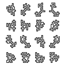
constellation definitions
Constellations were manually defined. Each constellation has a name and abbreviation (first 3 characters unless longer is required to uniquely specify it). Shown next is the number of stars used to define the constellation and their names, as appear in the star catalogue file above. Next is the number of edges and the star pairs that define the edges of the constellation. The edges are not in any particular order and have no direction. Any spaces in names are encoded with _.
DOWNLOAD

# idx n_stars n_edges name abbrev stars edges
 ...
 2  3  3                   alaotra     ala blts,btosf,cbkbw btosf-cbkbw,blts-btosf,blts-cbkbw
 3  4  4                 alloperla     all ghyr,pwkn,ssrx,ugwt pwkn-ssrx,pwkn-ghyr,ugwt-pwkn,ssrx-ghyr
 4  2  1                   aplonis     apl cbocd,rllm rllm-cbocd
 ...
You can use this file to quickly search for certain shapes. For example, triangular constellations are those that have 3 stars and 3 edges.
> grep " 3  3" constellations.def.txt
 2  3  3                   alaotra     ala blts,btosf,cbkbw btosf-cbkbw,blts-btosf,blts-cbkbw
16  3  3                   camptor    camp benxf,bqvh,bwqed bqvh-benxf,bwqed-bqvh,bwqed-benxf
26  3  3                  desmodus     des bfnqu,mork,zwzy bfnqu-mork,zwzy-bfnqu,zwzy-mork
27  3  3                ectopistes     ect bopmt,cbquf,wmnw cbquf-bopmt,wmnw-cbquf,wmnw-bopmt
30  3  3                    hoopoe     hoo bpsop,bvmjh,tryh tryh-bvmjh,bpsop-tryh,bpsop-bvmjh
31  3  3                      huia     hui ccteo,xbvq,yqet xbvq-yqet,ccteo-xbvq,ccteo-yqet
39  3  3               malpaisomys     mal bucqd,likq,nqn nqn-bucqd,likq-nqn,likq-bucqd
41  3  3                   mariana     mar gmps,jydb,pcjx pcjx-gmps,jydb-pcjx,jydb-gmps
49  3  3          palaeoaldrovanda     pal bedae,oife,saz bedae-saz,oife-bedae,oife-saz
63  3  3                    rhynia     rhy bpviv,cenuk,hivz bpviv-hivz,cenuk-bpviv,cenuk-hivz
65  3  3                  silphium     sil bjesg,bmquw,bpxia bmquw-bpxia,bjesg-bmquw,bjesg-bpxia
69  3  3                   tadorna     tad bukqe,cbtrx,epdx cbtrx-epdx,bukqe-cbtrx,bukqe-epdx
72  3  3                 traversia     tra fcnw,fywb,puib fywb-fcnw,puib-fywb,puib-fcnw
80  3  3                  yersinia     yer colq,ibls,zgvy ibls-zgvy,colq-ibls,colq-zgvy
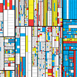
constellation boundaries
The boundaries were manually defined. Shown here, for each constellation, is the constellation's area, perimeter center and boundary `(x,y)` pairs, delimited by : and represent a closed polygon that encloses the constellation's stars.
All values are longitude and latitude. The three constellations listed below are ones with smallest area.
DOWNLOAD

# abbrev area perimeter centroid_xy boundary_xy_pairs

...
com 74.83 34.96 -102.50,26.25 -100.00,30.00:-102.50,30.00:-105.00,30.00:-107.50,30.00:-107.50,27.50:
			      -107.50,25.00:-107.50,22.51:-105.00,22.51:-102.50,22.51:-100.00,22.51:
			      -97.51,22.51:-97.51,25.00:-97.51,27.50:-97.51,30.00:-100.00,30.00
pal 50.02 30.00 3.43,-40.93 5.00,-37.49:2.50,-37.49:0.00,-37.49:0.00,-40.00:0.00,-42.50:0.00,-45.00:
			    2.50,-45.00:5.00,-45.00:5.00,-42.50:7.49,-42.50:7.49,-40.00:7.49,-37.49:5.00,-37.49
sil 37.57 25.02 115.00,-51.25 115.00,-47.50:112.49,-47.50:112.49,-50.00:112.49,-52.49:112.49,-55.00:
    	  		      115.00,-55.00:117.50,-55.00:117.50,-52.49:117.50,-50.00:117.50,-47.50:115.00,-47.50
The boundary polygons abut but do not overlap and they cover the entire sky. There is one polygon per consetllation. The total area of all constellations is `360 × 180 = 36800`.
constellation star membership
This is a list of all the stars on the chart and their constellation membership. A star is considered to be in a constellation if it falls within the constellation boundary.
The `i` and `j` indexes give the relative brightness of the star on the map and in the constellation, respectively. If a star is used to define the constellation edges it gets a + otherwise -.
DOWNLOAD

# abbreviation star i j mapp on_edge?
     aep bkawv     35     0   1.34 +
     aep   gql     65     1   1.63 +
     aep cavix     72     2   1.71 +
     aep bqxvm    137     3   2.25 +
     aep  tjow    158     4   2.31 +
     aep beelq    176     5   2.39 +
...
     yer  jjlj  39365   412   7.24 -
     yer bgswm  39464   413   7.24 -
     yer  ittu  39546   414   7.24 -
     yer  wakp  39556   415   7.24 -
     yer bedks  39667   416   7.25 -
     yer  gxzo  39817   417   7.25 -
To lookup the 10 brightest stars, sort on the i index. Here we see that megal (Megalodon) has the brightest star in the sky, jkxo with apparent magnitude `-2.05`. The next two brighest stars are in mam (Mammuthus) and ara (Araucaria).
> cat constellations.stars.txt | sort -n +2 -3 | head -10
   megal  jkxo      0     0  -2.05 +
     mam btsqy      1     0  -0.73 +
     ara ccijs      2     0  -0.38 +
     rap btaum      3     0   0.26 +
     urs bxlss      4     0   0.26 +
     tec bgrdk      5     0   0.43 +
     cop  itwr      6     0   0.45 +
     ara  mrvq      7     1   0.54 +
     phe  loju      8     0   0.54 +
     mam bhlbw      9     1   0.55 +
To get a list of the brightest star in each constellation, just search for " 0 ". Below I show this list sorted by brightness.
> cat constellations.stars.txt | grep " 0 "| sort -n +4 -5
   megal  jkxo      0     0  -2.05 +
     mam btsqy      1     0  -0.73 +
     ara ccijs      2     0  -0.38 +
     rap btaum      3     0   0.26 +
     urs bxlss      4     0   0.26 +
     tec bgrdk      5     0   0.43 +
     cop  itwr      6     0   0.45 +
     phe  loju      8     0   0.54 +
     kel bnhwx     11     0   0.59 +
     spe  rtep     13     0   0.71 +
     ...
     nes  vxou    299     0   2.80 -
     aur bmjvf    307     0   2.81 +
     tra  puib    318     0   2.83 +
     pip  cecq    358     0   2.91 +
     pal  oife    389     0   2.97 +
     swa   gvr    463     0   3.12 +
     hui ccteo    485     0   3.17 +
     ple bzqur    506     0   3.20 +
     com  ygrn    875     0   3.64 +
     car  yjkn    933     0   3.68 +
For example, tec (Tecopa) has bgrdk as its brightest star, which is 6th brightest in the sky with an apparent magnitude of 0.43.
The constellation whose brightest star is dimmest of all first brightest stars is car (Caracara). Its brightest star is yjkn which is 934th brightest in the sky with an apparent magnitude of 3.68.
To get the number of stars in each constellation, just add the number of times the constellation abbreviation appears. Bron has the most stars of any constellation, more than twice as many as the next one, archaeo (Archaeopteryx). Both car (Caracara) and por (Porzana) have only 7 stars each, the fewest of all constellations.
   5230 bro
   2287 archaeo
   2205 thy
   2155 kim
   1838 archaea
   1789 came
   1768 ard
...
     20 megal
     19 swa
     17 mar
     12 rhy
      8 sil
      7 por
      7 car
constellation names, stories and links
The constellations are in no particular order in this file.
DOWNLOAD

# constellation name
# hemisphere (n north, s south, b both)
# common name
# Latin name
# extinction date
# URL
# optional story

aplonis
n
mysterious bird of Ulieta
Aplonis ulietensis
1774-1850
https://en.wikipedia.org/wiki/Raiatea_starling

desmodus
n
Giant Vampire Bat
Desmodus draculae
Pleistocene or early Holocene
https://www.thoughtco.com/recently-extinct-shrews-bats-and-rodents-1092147
It is thought that each night Desmodus flies up against the dome of the sky, looking for a way to escape.

...
Nasa to send our human genome discs to the Moon
We'd like to say a ‘cosmic hello’: mathematics, culture, palaeontology, art and science, and ... human genomes.


Comparing classifier performance with baselines
All animals are equal, but some animals are more equal than others. —George Orwell
This month, we will illustrate the importance of establishing a baseline performance level.
Baselines are typically generated independently for each dataset using very simple models. Their role is to set the minimum level of acceptable performance and help with comparing relative improvements in performance of other models.

Unfortunately, baselines are often overlooked and, in the presence of a class imbalance5, must be established with care.
Megahed, F.M, Chen, Y-J., Jones-Farmer, A., Rigdon, S.E., Krzywinski, M. & Altman, N. (2024) Points of significance: Comparing classifier performance with baselines. Nat. Methods 20.
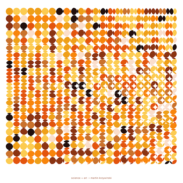
Happy 2024 π Day—
sunflowers ho!
Celebrate π Day (March 14th) and dig into the digit garden. Let's grow something.

How Analyzing Cosmic Nothing Might Explain Everything
Huge empty areas of the universe called voids could help solve the greatest mysteries in the cosmos.
My graphic accompanying How Analyzing Cosmic Nothing Might Explain Everything in the January 2024 issue of Scientific American depicts the entire Universe in a two-page spread — full of nothing.

The graphic uses the latest data from SDSS 12 and is an update to my Superclusters and Voids poster.
Michael Lemonick (editor) explains on the graphic:
“Regions of relatively empty space called cosmic voids are everywhere in the universe, and scientists believe studying their size, shape and spread across the cosmos could help them understand dark matter, dark energy and other big mysteries.
To use voids in this way, astronomers must map these regions in detail—a project that is just beginning.
Shown here are voids discovered by the Sloan Digital Sky Survey (SDSS), along with a selection of 16 previously named voids. Scientists expect voids to be evenly distributed throughout space—the lack of voids in some regions on the globe simply reflects SDSS’s sky coverage.”
voids
Sofia Contarini, Alice Pisani, Nico Hamaus, Federico Marulli Lauro Moscardini & Marco Baldi (2023) Cosmological Constraints from the BOSS DR12 Void Size Function Astrophysical Journal 953:46.
Nico Hamaus, Alice Pisani, Jin-Ah Choi, Guilhem Lavaux, Benjamin D. Wandelt & Jochen Weller (2020) Journal of Cosmology and Astroparticle Physics 2020:023.
Sloan Digital Sky Survey Data Release 12
Alan MacRobert (Sky & Telescope), Paulina Rowicka/Martin Krzywinski (revisions & Microscopium)
Hoffleit & Warren Jr. (1991) The Bright Star Catalog, 5th Revised Edition (Preliminary Version).
H0 = 67.4 km/(Mpc·s), Ωm = 0.315, Ωv = 0.685. Planck collaboration Planck 2018 results. VI. Cosmological parameters (2018).
constellation figures
stars
cosmology
Error in predictor variables
It is the mark of an educated mind to rest satisfied with the degree of precision that the nature of the subject admits and not to seek exactness where only an approximation is possible. —Aristotle
In regression, the predictors are (typically) assumed to have known values that are measured without error.
Practically, however, predictors are often measured with error. This has a profound (but predictable) effect on the estimates of relationships among variables – the so-called “error in variables” problem.

Error in measuring the predictors is often ignored. In this column, we discuss when ignoring this error is harmless and when it can lead to large bias that can leads us to miss important effects.
Altman, N. & Krzywinski, M. (2024) Points of significance: Error in predictor variables. Nat. Methods 20.
Background reading
Altman, N. & Krzywinski, M. (2015) Points of significance: Simple linear regression. Nat. Methods 12:999–1000.
Lever, J., Krzywinski, M. & Altman, N. (2016) Points of significance: Logistic regression. Nat. Methods 13:541–542 (2016).
Das, K., Krzywinski, M. & Altman, N. (2019) Points of significance: Quantile regression. Nat. Methods 16:451–452.
Convolutional neural networks
Nature uses only the longest threads to weave her patterns, so that each small piece of her fabric reveals the organization of the entire tapestry. – Richard Feynman
Following up on our Neural network primer column, this month we explore a different kind of network architecture: a convolutional network.
The convolutional network replaces the hidden layer of a fully connected network (FCN) with one or more filters (a kind of neuron that looks at the input within a narrow window).
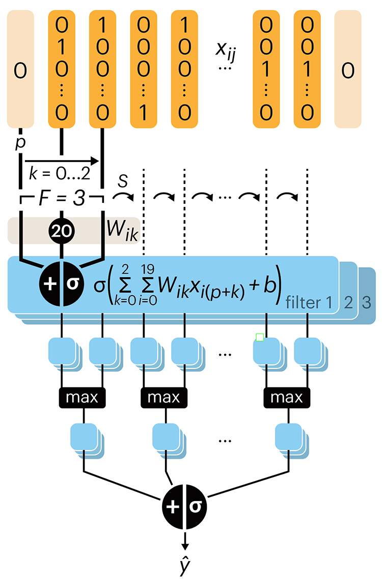
Even through convolutional networks have far fewer neurons that an FCN, they can perform substantially better for certain kinds of problems, such as sequence motif detection.
Derry, A., Krzywinski, M & Altman, N. (2023) Points of significance: Convolutional neural networks. Nature Methods 20:1269–1270.
Background reading
Derry, A., Krzywinski, M. & Altman, N. (2023) Points of significance: Neural network primer. Nature Methods 20:165–167.
Lever, J., Krzywinski, M. & Altman, N. (2016) Points of significance: Logistic regression. Nature Methods 13:541–542.