If you are interested in color, explore my other color tools, Brewer palettes resources, color blindness palettes and math and an exhausting list of 10,000 color names for all those times you couldn't distinguish between tan hide, sea buckthorn, orange peel, west side, sunshade, california and pizzaz.

Designing for Color blindness

Color choices and transformations for deuteranopia and other afflictions

Here, I help you understand color blindness and describe a process by which you can make good color choices when designing for accessibility.

The opposite of color blindness is seeing all the colors and I can help you find 1,000 (or more) maximally distinct colors.

You can also delve into the mathematics behind the color blindness simulations and learn about copunctal points (the invisible color!) and lines of confusion.

Maximally distinct colors

Color blindness is the inability to distinguish colors. The converse of this is a set of maximual distinct colors — interesting in its own right and subject of this section.

Below I also provide helpful diagrams that visualize how color differences vary. These show the difference between two modern formulae for color differences: `\Delta E_{94}` and `\Delta E_{00}`.

▲ A set of `N=1000` maximally distinct colors (download list) obtained by k-means clustering 815,267 colors that evenly sample the sRGB gamut. Distance metric is `\Delta E_{00}`.

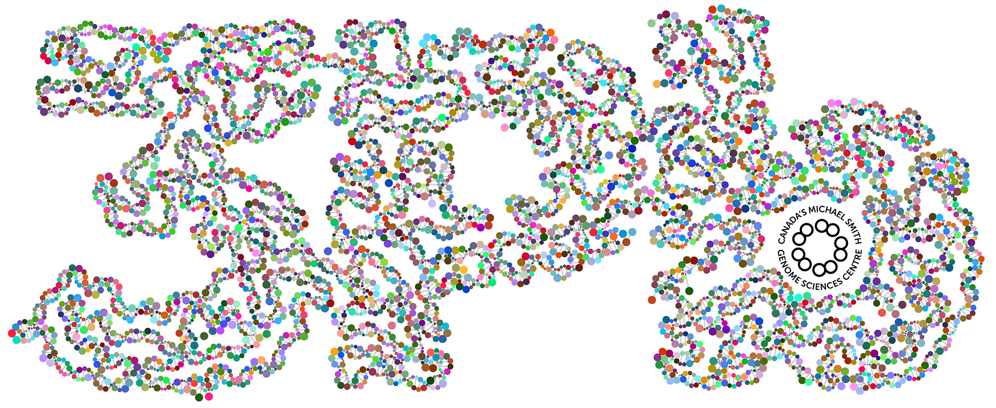
When we had reached 3 petabases milestone in our sequencing, I made a graphic of a DNA double helix of 3,000 base pairs that wound into the shape of "3Pb". I wanted to color each base on a strand with a different reasonably saturated and bright color — the base on the opposite strand would be its RGB inverse.

I didn't want just different — I wanted maximally distinct. While it's very easy to pick any number of RGB colors that are different, it's trickier to make sure that they're all as different from each other as possible.

▲ A double-helix of 3,000 base pairs to commemorate 3 petabases sequenced at Canada's Michael Smith Genome Sciences Center. Each of the 3,000 bases on a strand has a maximally distinct color and its complement is the RGB inverse. The RGB inverses are not maximally distinct.

Here, I outline a method for selecting such a large number of distinct colors and provide these color sets for you to download. You can pick anywhere a set of anywhere from `N=20` to `5,000` maximally distinct colors.

The selection method described below is essentially the same as offered by the excellent iwanthue project, which provides an excellent visual tutorial of the idea of color differences. Unfortunately, the tool timed out when attempting to find 3,000 different colors, so I thought I'd generate a set myself.

These sets are from a subset of the 815,267 colors (see methods) limited to `L = 20-80` and `C \ge 20`. Extremely bright colors (e.g. pure yellows) are not included. For sets drawn from the full complement of 815,267 colors, see below.

Shown below are sets of `N=5-50` maximally distinct colors. The first swatch in the set is the one closest to pure RGB red (255,0,0). The next swatch is the first swatche's closest `\Delta E` neighbour and so on — the order is sensitive to small changes in color difference as well as the color of the first patch so it can be quite different for each set. The average `\Delta E` between closest neighbours is shown on the left — the fewer the colors, the larger the color clusters from which they were sampled and thus the larger the `\Delta E`.

▲ Sets of `N=5-100` maximally distinct colors and the average `\Delta E` between closest colors in the set.

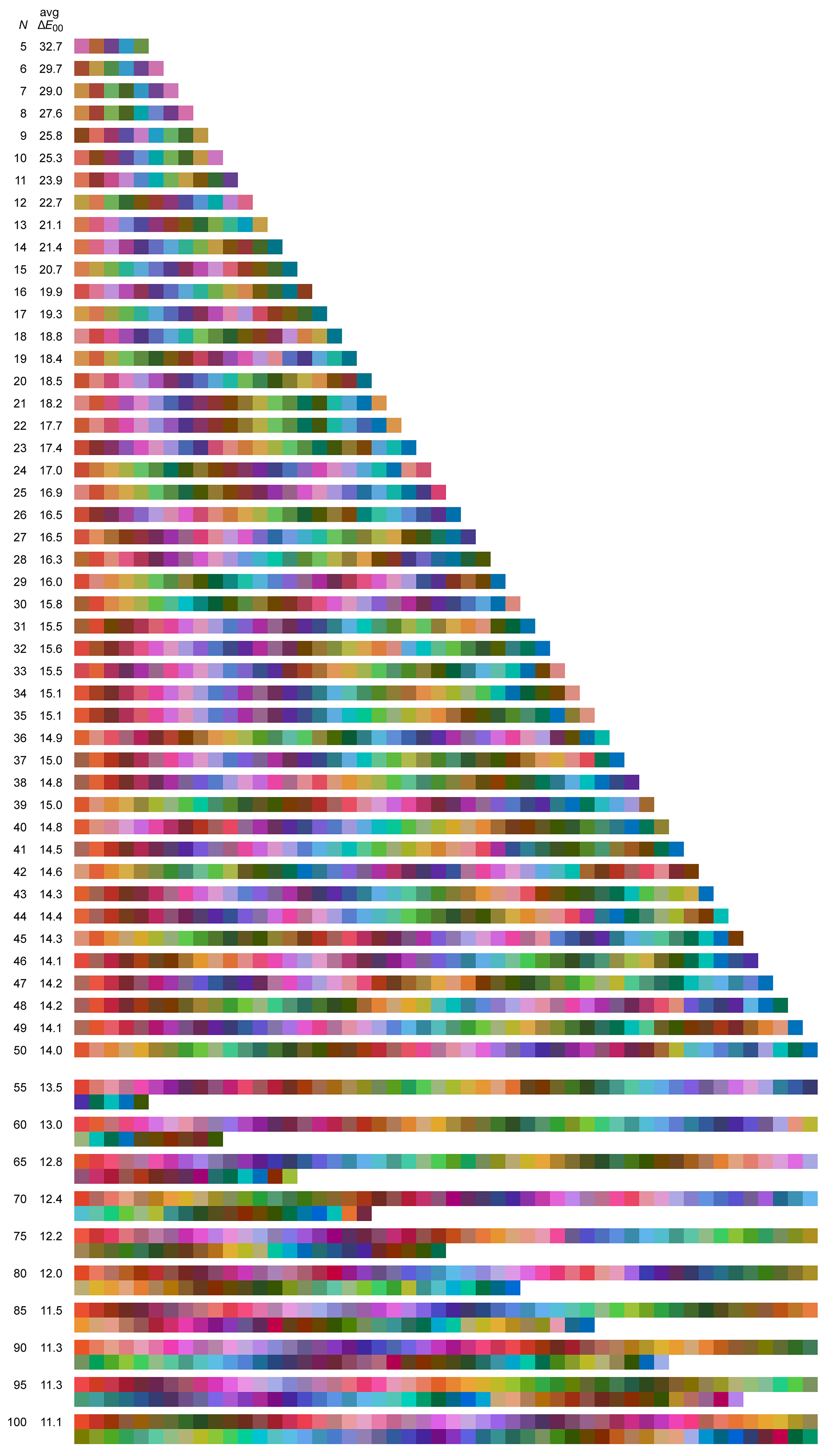
The k-means clustering is stochastic — each time it's run you get a slightly different result as the algorithm tries to search for a global maximum (it won't find it but it will find many local minima).

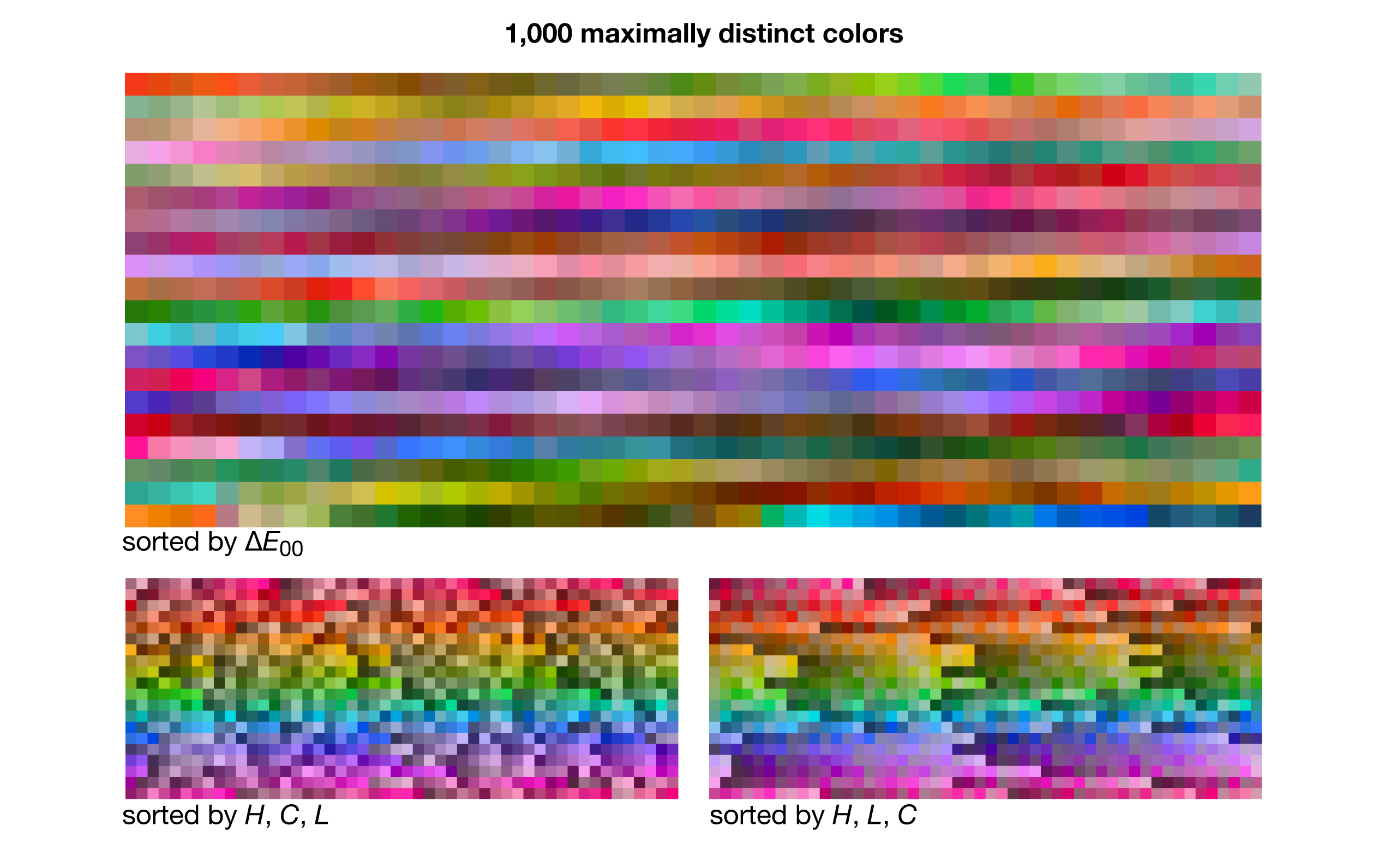
Some larger sets of maximally distinct colors are shown below, ordered by either `\Delta E` or LCH.

▲ Sets of `N` maximally distinct colors and the average `\Delta E` between closest colors in the set. (left) Within a set, swatches are sorted by `\Delta E` with the previous swatch. (right) Within a set, swatches are sorted by hue, chroma and luminance.

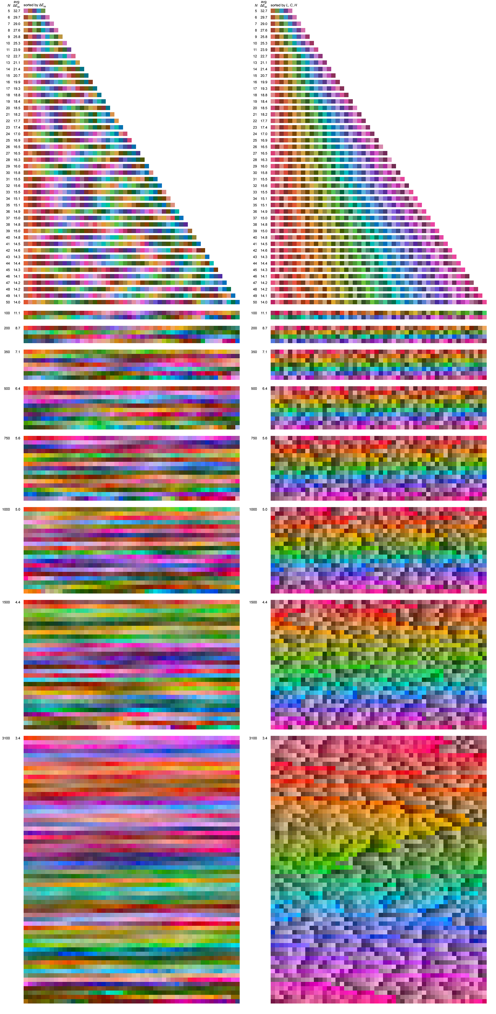
The benefit of sorting by closest neighbours is that you can see the extent to which the color space is sampled — as the set of colors grows, a color's nearest neighbour becomes more and more similar. Sorting by LCH (hue first, then chroma, then luminance — each rounded off to nearest 5) helps to see how many colors from a given part of the hue wheel are chosen. For example, note how there's generally more reds than blues.

A more in-depth description of color differences is below. For the color selection I use CIE00 (`\Delta E_{00}`) but CIE94 would probably be just as good (and faster).

The process of selecting this set of maximally distinct colors starts with sampling all LCH colors in the range `LCH = [0,100] \times [0,100] \times [0,359]` in steps of `0.5` in each dimension. This creates an initial set of 28.8 million colors — more than 24-bit RGB colors. So, too many!

First, I eliminate all colors that have identical integer RGB values. This leaves me with 6.1 million colors.

Then, to make the analysis more practical, I find a subset of the 6.1 million by eliminating any colors that already have a color within `\Delta E_{00} < 0.5` in the set. Remember that neither Lab (and therefore LCH aren't perceptually uniform) so among the 6.1 million colors, some will be more similar to each other than others.

This filtering gives me 815,267 RGB colors (download list). In this set, the average distance between nearest color neighbours (`\Delta E`) is 0.54 and 99% of the `\Delta E < 0.8`. Only 683 (<0.1%) of colors have a nearest neighbour with `\Delta E > 1` and 41 colors have a nearest neighbour with `\Delta E > 2`. These are in areas where `\Delta E` changes quickly with small changes in RGB. For example the two colors (46,0,0) and (47,0,0) have a `\Delta E = 2.0` but only vary by `\Delta R = 1`.

I'm sticking to integer RGB values — given that I'm sampling a very large number of colors, the few places where carrying a decimal would even out the local sampling is negligible. As well, my original purpose of creating these color sets was for design and most applications (Photoshop, Illustrator, etc) limit you to integer RGB.

To find the set of `N` maximally distinct colors, I apply k-means clustering using `\Delta E_{00}` as the distance metric. For sets `N = 5-100` I run k-means 100 times and choose the one with lowest error. For `N=110-200` I run k-means 25 times and for `N=225-1000` I run it 5 times. For `N>1000` I run k-means only once.

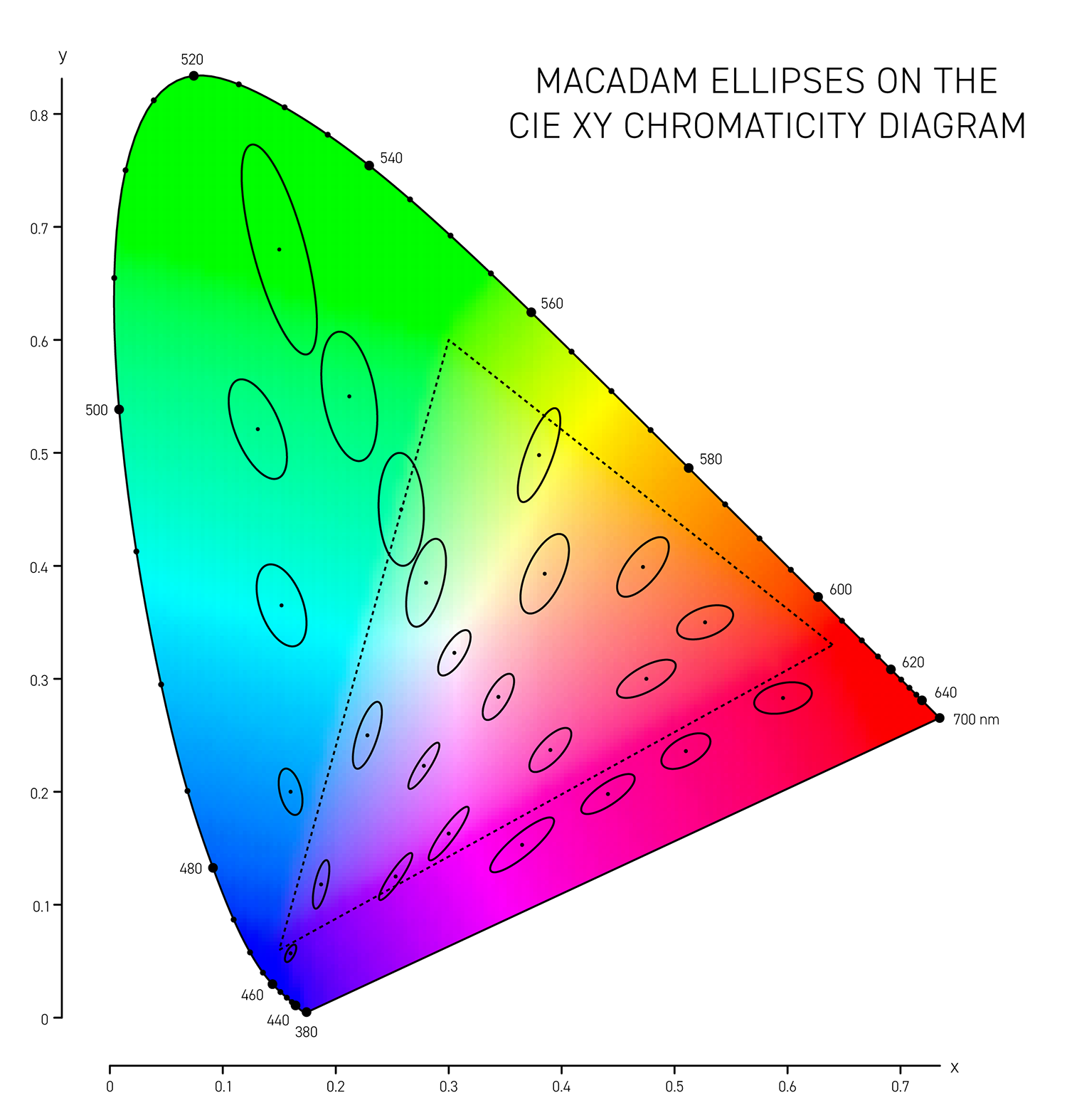
In 1942 D.L. MacAdam published Visual sensitivities to color differences in daylight in which he demarcated regions of indistinguishable colors in CIE `xy` chromaticity space at 25 locations — these form the MacAdam ellipses (download ellipse positions).

▲ MacAdam ellipses (shown here enlarged by factor of 10×) represent the limit of color discrimination.

The difference between colors is called delta E (`\Delta E`) and is expressed by a number of different formulas — each slightly better at incorporating how we perceive color differences.

The simplest is the CIE76 `\Delta E` and this is the Euclidian distance between two colors in the CIE Lab color space. The Lab space is not perceptually uniform so this formula, while doing a reasonable job overall, doesn't distinguish between the extent to which we see differences in colors that are very saturated (saturation in Lab is called chroma `C = \sqrt{a^2+b^2}`). A difference of `\Delta E_{76} = 2.3` is called the JND (just noticeable difference) and is considered the limit of color discrimination (on average).

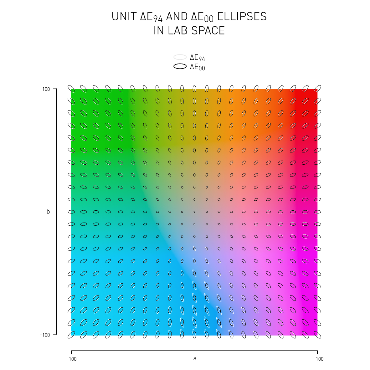
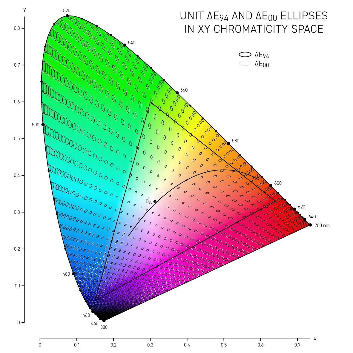
More sophisticated versions of `\Delta E` such as CIE94 and CIE00 attempt to address the non-uniformity of Lab space and with the aim to have a `\Delta E = 1` corresponds to a just noticeable difference (JND). Below, I show unit ellipses for CIE94 and CIE00 in Lab and `xy` chromaticity space — colors on the opposite side of an ellipse have a `\Delta E = 1`.

CIE94 and CIE00 are very similar to each other, except for blues and purples, where `\Delta E_{00}` ellipses are more eccentric and in the saturated greens where they are a little wider. In both cases the ellipses point in the direction of saturation — this corresponds to the fact that we discriminate hue better than saturation in Lab space. CIE00 is a more complicated calculation (and called by some an ugly calculation) and therefore slower — I'll guess that for most applications CIE94 is sufficient.

▲ Unit ellipses for `\Delta E_{94}` (black) and `\Delta E_{00}` (light grey, drawn below `\Delta E_{94}` ellipses) sampled at uniform points in Lab space. Where the light grey ellipses peek out from under black ones, the two `\Delta E` models vary. Note that `\Delta E_{00}` is most different in the blues and purples and to a lesser extent in the saturated greens. The color of the background corresponds to a Lab luminance `L = 70` with a slight desaturation filter.

▲ Unit ellipses for `\Delta E_{94}` and `\Delta E_{00}` sampled at uniform points in Lab space and shown on the xy chromaticity diagram. Also shown are the sRGB gamut, D65 illuminant and Planckian locus.

For more details about color differences see Colour difference `\Delta E` — A survey by W.S. Mokrzycki and M. Tatol.