Designing for Color blindness
Color choices and transformations for deuteranopia and other afflictions
Here, I help you understand color blindness and describe a process by which you can make good color choices when designing for accessibility.
The opposite of color blindness is seeing all the colors and I can help you find 1,000 (or more) maximally distinct colors.
You can also delve into the mathematics behind the color blindness simulations and learn about copunctal points (the invisible color!) and lines of confusion.
Math of color blindness
contents
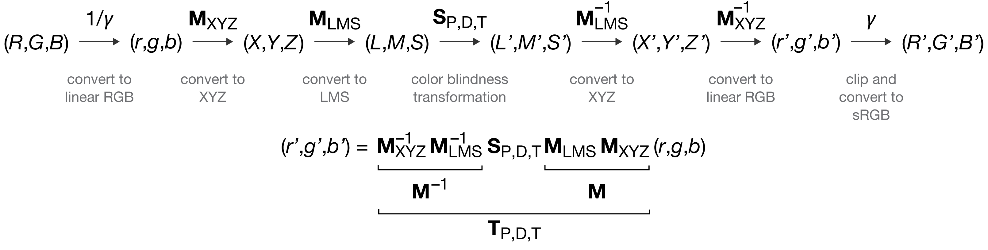
The transformations described here will allow you to simulate color blindness and apply conversions of the kind shown in the images below to your own work.
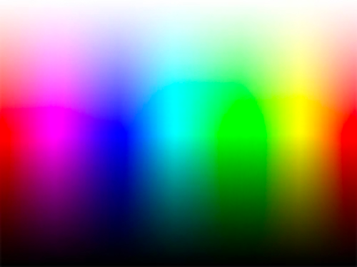
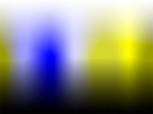
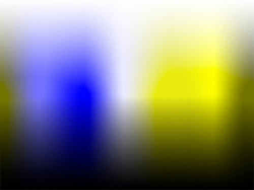
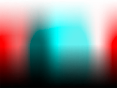

The conversion from RGB values to their color blindness equivalents for protanopia, deuteranopia and tritanopia consists of the following steps
- convert from sRGB to linear RGB
- convert from linear RGB to XYZ
- convert from XYZ to LMS
- apply color blindness transformation in LMS space
- convert from LMS to XYZ (inverse of #3)
- convert from XYZ to linear RGB (inverse of #2)
- convert from linear RGB to sRGB (clip and inverse of #1)
The greyscale conversion for achromatopsia does not require the XYZ and LMS steps. We can go straight to `Y`.
- convert from sRGB to linear RGB
- `Y = 0.02126r + 0.7152g + 0.0722b`
- convert from linear RGB to sRGB (inverse of #1)
The details of each of the steps are shown below. If you just want the `\mathbf{T}` matrices, scroll down to the bottom or download the code.
Depending on the implementation, this process may have an additional step that reduces the color domain (e.g. step 2 in Viénot, Brettel & Mollon, 1999). This makes sure that none of the transformed colors are outside of the sRGB domain. Here, I instead of doing this I just clip the transformed colors at the end. This simplifies the process and (my sense is that) the difference is negligible.
Different simulators will yield slightly different results, too.
The RGB input color is `\{R,G,B\} = \{ V \in [0,255] \}` and assumed to be sRGB. This is first linearized with `\gamma = 2.4` to obtain `\{r,g,b\} = \{ v \in [0,1] \}`. $$v = \begin{cases} \dfrac{V/255}{12.92} & \text{if $V/255 \le 0.04045$} \\[2ex] \left({\dfrac{V/255+0.055}{1.055}}\right)^\gamma & \text{otherwise} \end{cases} $$
Next, convert the linearized `(r,g,b)` to XYZ by multiplying by `\mathbf{M}_\textrm{XYZ}`. $$ \left[ \begin{matrix} X \\Y \\Z \end{matrix} \right] = \underbrace{ \left[ \begin{matrix} 0.4124564 & 0.3575761 & 0.1804375 \\0.2126729 & 0.7151522 & 0.0721750 \\0.0193339 & 0.1191920 & 0.9503041 \end{matrix} \right] }_{\mathbf{M}_\textrm{XYZ}} \left[ \begin{matrix} r \\g \\b \end{matrix} \right] $$
Multiply by `\mathbf{M}_\textrm{LMSD65}` to convert XYZ to LMS. This matrix is normalized to the D65 illuminant, which will ensure that greys will be preserved.
The LMS (long, medium, short) is a color space which represents the response of the three types of cones of the human eye, named for their sensitivity peaks at long (560 nm, red) medium (530 nm, green), and short (420 nm, blue) wavelengths. $$ \left[ \begin{matrix} L \\ M \\ S \end{matrix} \right] = \underbrace{ \left[ \begin{matrix} 0.4002 & 0.7076 & -0.0808 \\ -0.2263 & 1.1653 & 0.0457 \\ 0 & 0 & 0.9182 \end{matrix} \right] }_{\mathbf{M}_\textrm{LMSD65}} \left[ \begin{matrix} X \\ Y \\ Z \end{matrix} \right] $$
If for some reason you don't want to normalize to D65, you would use `\mathbf{M}_\textrm{LMS}` below but whites will now appear pinkish. $$ \left[ \begin{matrix} L \\ M \\ S \end{matrix} \right] = \underbrace{ \left[ \begin{matrix} 0.38971 & 0.68898 & -0.07868 \\ -0.22981 & 1.18340 & 0.04641 \\ 0 & 0 & 1 \end{matrix} \right] }_{\mathbf{M}_\textrm{LMS}} \left[ \begin{matrix} X \\ Y \\ Z \end{matrix} \right] $$
There are other XYZ to LMS matrices and the R code lists them all. Below this section, I show the dichromacy transformations for each of these XYZ-LMS matrices.
Now that we have the RGB color represented in LMS space, we can correct for color receptor dysfunction in this space, since color blindness affects one of the L, M or S receptors.
I show the calculations here in a lot of detail—they're not as complicated as things look. Once you understand what's happening for one of the color blindness types, the other two are analogously treated.
Each of the color blindness types will have its own correction matrix `\mathbf{S}`. $$ \left[ \begin{matrix} L' \\ M' \\ S' \end{matrix} \right] = \mathbf{S} \left[ \begin{matrix} L \\ M \\ S \\ \end{matrix} \right] $$
This matrix is the identity matrix with the row for the malfunctioning receptor (e.g. S for protanopia) replaced by two free parameters `a` and `b`. $$ \begin{align} \mathbf{S}_\textrm{protanopia} & = \left[ \begin{matrix} 0 & a & b \\ 0 & 1 & 0 \\ 0 & 0 & 1 \end{matrix} \right] \\ \mathbf{S}_\textrm{deuteranopia} & = \left[ \begin{matrix} 1 & 0 & 0 \\ a & 0 & b \\ 0 & 0 & 1 \end{matrix} \right] \\ \mathbf{S}_\textrm{tritanopia} & = \left[ \begin{matrix} 1 & 0 & 0 \\ 0 & 1 & 0 \\ a & b & 0 \end{matrix} \right] \end{align} $$
The reason why these matrices have this format is so that we can satisfy two conditions. First, we expect that one of the `rgb` primaries won't be affected, depending on the color blindness type. For protanopia and deuteranopia this is blue and for tritanopia this is red. Second, this matrix should not affect how white appears—if one of the rows was just zero then white would be altered.
If we set `\mathbf{M} = \mathbf{M}_\textrm{LMSD65} \mathbf{M}_\textrm{XYZ}` then these conditions (using the blue case for protanopia) can be expressed as $$ \mathbf{S}_\textrm{protanopia} \mathbf{M} \left[ \begin{matrix} 0 \\ 0 \\ 1 \end{matrix} \right] = \mathbf{M} \left[ \begin{matrix} 0 \\ 0 \\ 1 \end{matrix} \right] = \left[ \begin{matrix} L_b \\ M_b \\ S_b \end{matrix} \right] $$ $$ \mathbf{S}_\textrm{protanopia} \mathbf{M} \left[ \begin{matrix} 1 \\ 1 \\ 1 \end{matrix} \right] = \mathbf{M} \left[ \begin{matrix} 1 \\ 1 \\ 1 \end{matrix} \right] = \left[ \begin{matrix} L_0 \\ M_0 \\ S_0 \end{matrix} \right] $$
where `(L_b,M_b,S_b)` of the primary that is not affected (e.g. blue) and `(L_0,M_0,S_0)` are the LMS coordinates of white. These two coordinates are eigenvectors of `\mathbf{S}_\textrm{protanopia}` with an eigenvalue of `\lambda=1`. Using the form for `\mathbf{S}_\textrm{protanopia}`, these lead to the following equations $$ \begin{align} a M_b + b S_b & = L_b \\a M_0 + b S_0 & = L_0 \end{align} $$
which can be written as $$ \left[ \begin{matrix} a \\b \end{matrix} \right]_\textrm{protanopia} = { \left[ \begin{matrix} M_b & S_b \\M_0 & S_0 \end{matrix} \right] }^{-1} \left[ \begin{matrix} L_b \\L_0 \end{matrix} \right] $$
For deuteranopia and tritanopia the calculation of `a` and `b` is analogous, except that because now `a` and `b` change position in `\mathbf{S}`, the equations are slightly different. $$ \left[ \begin{matrix} a \\b \end{matrix} \right]_\textrm{deuteranopia} = { \left[ \begin{matrix} L_b & S_b \\L_0 & S_0 \end{matrix} \right] }^{-1} \left[ \begin{matrix} M_b \\M_0 \end{matrix} \right] $$
and for tritanopia (here `(L_r,M_r,S_r)` refers to the coordinates of red). $$ \left[ \begin{matrix} a \\b \end{matrix} \right]_\textrm{tritanopia} = { \left[ \begin{matrix} L_r & M_r \\L_0 & M_0 \end{matrix} \right] }^{-1} \left[ \begin{matrix} S_r \\S_0 \end{matrix} \right] $$
Using the following LMS coordinates (calculated by linearizing the corresponding RGB values and then muptiplying by `\mathbf{M}`) $$ \begin{align} \left[ \begin{matrix} L_0 \\ M_0 \\ S_0 \end{matrix} \right] & = \left[ \begin{matrix} 1 \\ 0.999683 \\ 0.9997637 \end{matrix} \right] \\ \left[ \begin{matrix} L_b \\ M_b \\ S_b \end{matrix} \right] & = \left[ \begin{matrix} 0.04649755 \\ 0.08670142 \\ 0.87256922 \end{matrix} \right] \\ \left[ \begin{matrix} L_r \\ M_r \\ S_r \end{matrix} \right] & = \left[ \begin{matrix} 0.31399022 \\ 0.15537241 \\ 0.01775239 \end{matrix} \right] \end{align} $$
Using protanopia as the example $$ \begin{align} \left[ \begin{matrix} a \\b \end{matrix} \right]_\textrm{protanopia} & = { \left[ \begin{matrix} 0.08670142 & 0.87256922 \\0.999683 & 0.9997637 \end{matrix} \right] }^{-1} \left[ \begin{matrix} 0.04649755 \\1 \end{matrix} \right] \\ & = \left[ \begin{matrix} -1.27219 & 1.1103359 \\1.27245 & -0.1103267 \end{matrix} \right] \left[ \begin{matrix} 0.04649755 \\1 \end{matrix} \right] \\ & = \left[ \begin{matrix} 1.05118294 \\-0.05116099 \end{matrix} \right] \end{align} $$
The `(a,b)` calculations for deuteranopia and tritanopia are analogous and once they're done we can write the correction matrices as $$ \left[ \begin{matrix} L' \\ M' \\ S' \end{matrix} \right] = \underbrace{ \left[ \begin{matrix} 0 & 1.05118294 & -0.05116099 \\ 0 & 1 & 0 \\ 0 & 0 & 1 \end{matrix} \right] }_{\mathbf{S}_\textrm{protanopia}} \left[ \begin{matrix} L' \\ M' \\ S' \end{matrix} \right] $$ $$ \left[ \begin{matrix} L' \\ M' \\ S' \end{matrix} \right] = \underbrace{ \left[ \begin{matrix} 1 & 0 & 0 \\ 0.9513092 & 0 & 0.04866992 \\ 0 & 0 & 1 \end{matrix} \right] }_{\mathbf{S}_\textrm{deuteranopia}} \left[ \begin{matrix} L' \\ M' \\ S' \end{matrix} \right] $$ $$ \left[ \begin{matrix} L' \\ M' \\ S' \end{matrix} \right] = \underbrace{ \left[ \begin{matrix} 1 & 0 & 0 \\ 0 & 1 & 0 \\ -0.86744736 & 1.86727089 & 0 \end{matrix} \right] }_{\mathbf{S}_\textrm{tritanopia}} \left[ \begin{matrix} L' \\ M' \\ S' \end{matrix} \right] $$
These `(a,b)` values are for the D65-normalized XYZ-to-LMS matrix and will change if you use a different matrix. The R code calculates `(a,b)` for whatever matrix you provide.
Once the color blindness correction has been applied in LMS space, we convert back to XYZ using the inverse `\mathbf{M}_\text{LMSD65}^{-1}`. $$ \left[ \begin{matrix} X' \\ Y' \\ Z' \end{matrix} \right] = \underbrace{ \left[ \begin{matrix} 1.8600666 & -1.1294801 & 0.2198983 \\ 0.3612229 & 0.6388043 & 0 \\ 0 & 0 & 1.089087 \end{matrix} \right] }_{\mathbf{M}_\textrm{LMSD65}^{-1}} \left[ \begin{matrix} L' \\ M' \\ S' \end{matrix} \right] $$
If you used `\mathbf{M}_\textrm{LMS}` and didn't normalize to D65, then you'd use its inverse `\mathbf{M}_\text{LMS}^{-1}` instead. $$ \left[ \begin{matrix} X' \\ Y' \\ Z' \end{matrix} \right] = \underbrace{ \left[ \begin{matrix} 1.9101968 & -1.1121239 & 0.2019080 \\ 0.3709501 & 0.6290543 & 0 \\ 0 & 0 & 1 \end{matrix} \right] }_{\mathbf{M}_\textrm{LMS}^{-1}} \left[ \begin{matrix} L' \\ M' \\ S' \end{matrix} \right] $$
Finally, one last matrix multiplication from XYZ back to linear RGB using `\mathbf{M}_\textrm{XYZ}^{-1}`. $$ \left[ \begin{matrix} r' \\ g' \\ b' \end{matrix} \right] = \underbrace{ \left[ \begin{matrix} 3.24045484 & -1.5371389 & -0.49853155 \\ -0.96926639 & 1.8760109 & 0.04155608 \\ 0.05564342 & -0.2040259 & 1.05722516 \end{matrix} \right] }_{\mathbf{M}_\textrm{XYZ}^{-1}} \left[ \begin{matrix} X' \\ Y' \\ Z' \end{matrix} \right] $$
The first step is now inverted to obtain the final sRGB values as perceived by someone with color blindness. $$V = \begin{cases} 255(12.92v) & \text{if $v \le 0.0031308$} \\[1ex] 255(1.055 v^{1/\gamma} - 0.055) & \text{otherwise} \end{cases} $$
Make sure to clip `v` to `[0,1]` before applying the final transformation back to sRGB.
The matrix multiplication steps can be written compactly as $$ \left[ \begin{matrix} r' \\ g' \\ b' \end{matrix} \right] = \mathbf{M}_\textrm{XYZ}^{-1} \mathbf{M}_\textrm{LMSD65}^{-1} \mathbf{S} \mathbf{M}_\textrm{LMSD65} \mathbf{M}_\textrm{XYZ} \left[ \begin{matrix} r \\ g \\ b \end{matrix} \right] = \mathbf{T} \left[ \begin{matrix} r \\ g \\ b \end{matrix} \right] $$
where `\mathbf{T}` is the product of all the matrices for a given color blindness correction `\mathbf{S}`, which are $$ \begin{align} \mathbf{T}_\textrm{protanopia} & = \left[ \begin{matrix} 0.170556992 & 0.829443014 & 0 \\ 0.170556991 & 0.829443008 & 0 \\ -0.004517144 & 0.004517144 & 1 \end{matrix} \right] \\ \mathbf{T}_\textrm{deuteranopia} & = \left[ \begin{matrix} 0.33066007 & 0.66933993 & 0 \\ 0.33066007 & 0.66933993 & 0 \\ -0.02785538 & 0.02785538 & 1 \end{matrix} \right] \\ \mathbf{T}_\textrm{tritanopia} & = \left[ \begin{matrix} 1 & 0.1273989 & -0.1273989 \\ 0 & 0.8739093 & 0.1260907 \\ 0 & 0.8739093 & 0.1260907 \end{matrix} \right] \\ \mathbf{T}_\textrm{achromatopsia} & = \left[ \begin{matrix} 0.2126 & 0.7152 & 0.0722 \\ 0.2126 & 0.7152 & 0.0722 \\ 0.2126 & 0.7152 & 0.0722 \end{matrix} \right] \end{align} $$
The matrices above use the LMSD65 XYZ-LMS conversion matrix.
Here I summarize all the `rgb` colorblindness tranformation matrices for each XYZ-LMS conversion matrix. The transformation for achromatopsia does not depend on how the XYZ-LMS conversion is done.
If colorblindness is partial (e.g. associated photoreceptors are present but either reduced in number of function), then the correction matrix is a linear combination of the total colorblindness correction matrix (e.g. `\mathbf{T}_\textrm{protanopia}`) and the identity matrix: `k\mathbf{T}_\textrm{protanopia}+(1-k)\mathbf{I}`, where `k=1` corresponds to total colorblindness and `k=0` is perfect color vision.
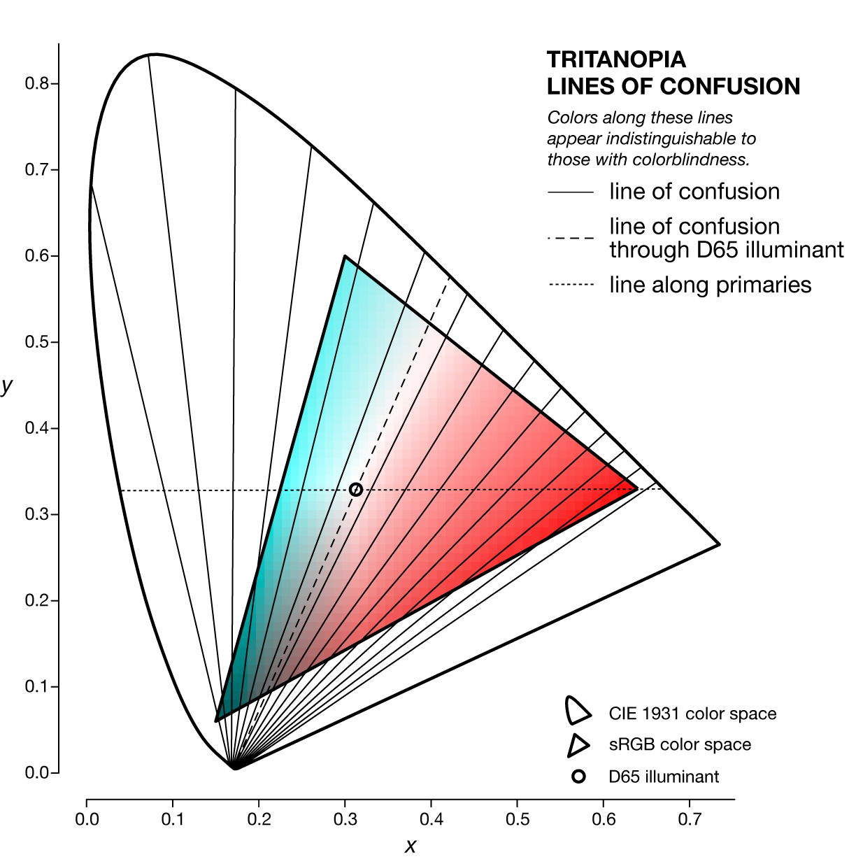
A line of confusion is the set of colors that appear identical to someone with colorblindness. Each kind of colorblindness has its own set of lines of confusion.
Lines of confusion can be nicely visualized in `xyY` color space, in which the chromaticity of a color is specified by `(x,y)` and the luminance by `Y`. This space is the projection of the `XYZ` color space onto the plane with the equation `X+Y+Z=`, which is the triangle made by the ends of the unit vectors in `XYZ` space (i.e. `[1,0,0],[0,1,0],[0,0,1]`).
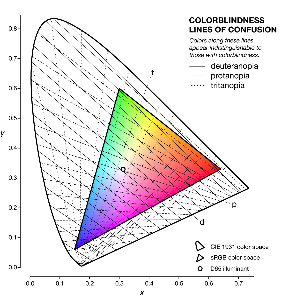
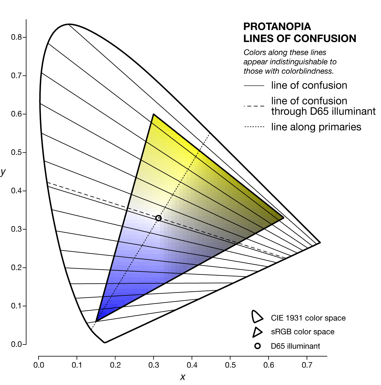
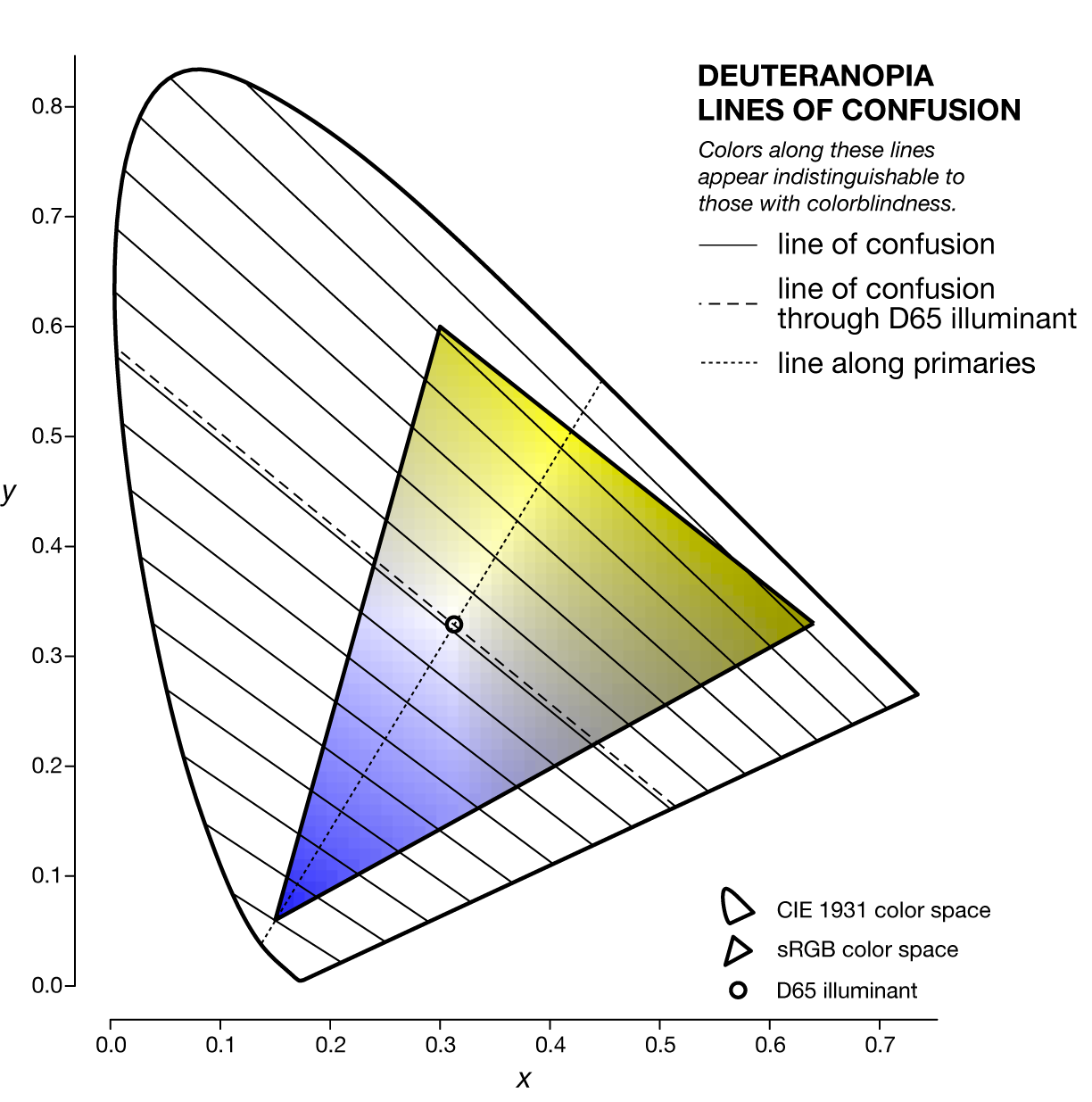
The specific line of confusion that passes through the white point divides the space into two hues. For example, for protanopes and deuteranopes these hues are blue and yellow but the line that divides the CIE space into the hues is slightly different. The figures below also show the line between the two colorblind primaries — the two colors that are not altered by the colorblindness (read below).
The nature of the lines of confusion can be understood in terms of the colorblindness transformation matrices described above. Recall that to convert an `[X,Y,Z]` color to its colorblind equivalent `[X',Y',Z']` we use $$ \left[ \begin{matrix} X' \\ Y' \\ Z' \end{matrix} \right] = \mathbf{M}^{-1}_{\textrm{LMSD65}} \mathbf{S_{\textrm{p,d,t}}} \mathbf{M}_{\textrm{LMSD65}} \left[ \begin{matrix} X \\ Y \\ Z \end{matrix} \right] = \mathbf{T_{\textrm{p,d,t}}} \left[ \begin{matrix} X \\ Y \\ Z \end{matrix} \right] $$
where `\mathbf{M}` is the transformation from `XYZ` to `LMS` and `\mathbf{S}` is the projection matrix in `LMS` space for a given colorblindness type. Above, I write the product of these three matrices as `\mathbf{T}_{\textrm{p,d,t}}`, with the subscript indicating the type of colorblindness.
For example, for deuteranopia, we have $$ \left[ \begin{matrix} X' \\ Y' \\ Z' \end{matrix} \right] = \mathbf{T}_{\textrm{d}} \left[ \begin{matrix} X \\ Y \\ Z \end{matrix} \right] = \left[ \begin{matrix} 0.3143898 & 0.5558777 & 0.08796059 \\ 0.3877631 & 0.6856102 & -0.04974820 \\ 0 & 0 & 0 \end{matrix} \right] \left[ \begin{matrix} X \\ Y \\ Z \end{matrix} \right] $$
Consider the eigenvectors `\mathbf{v}_\textrm{d}` and their corresponding eigenvalues `\lambda_\textrm{d}` of this matrix. The eigenvectors are the solution to the equation `(\mathbf{T}_{\textrm{d}} - \lambda_\textrm{d}\mathbf{I} )\mathbf{v}_\textrm{b} = 0`, which answers the question "what vectors are projected onto a multiple (the eigenvalue) of themselves?". The eigenvectors for deuteranopia are $$ \mathbf{v}_{\textrm{d},\lambda=1} = \left[ \begin{matrix} -0.62978663 \\ -0.77676818 \\ 0 \end{matrix} \right] \qquad \mathbf{v}_{\textrm{d},\lambda=1} = \left[ \begin{matrix} 0.06766092 \\ -0.07398814 \\ 0.99496188 \end{matrix} \right] \qquad \mathbf{v}_{\textrm{d},\lambda=0} = \left[ \begin{matrix} -0.8704299 \\ 0.4922923 \\ 0 \end{matrix} \right] $$
The first two eigenvectors have a unit eigenvalue `\lambda=1` and thus are transformed to themselves under the colorblind transformation. These correspond to the unique points in `XYZ` space that are perceived (if they are within the range of perceived colors & mdash; see below) identically by those with colorblindness and with normal vision. They form a basis of the `XYZ` subspace (which is a plane) of transformed colors — and can be considered as primaries, since someone with colorblindness can only perceive colors created in this plane (i.e. by mixing the primaries). Any color that is not on this plane will appear the same as some color on this plane — this is where the third eigenvector comes in.
The third eigenvector has a zero eigenvalue `\lambda=0`. It is therefore transformed to zero (i.e. black in an additive color space like `XYZ`). Thus, adding a multiple of this eigenvector to any color `XYZ` will not affect its colorblind transform — adding any amount of "no light" to any light does not change the light. Any point `\mathbf{X}` on the plane mentioned above can be moved along the parameteric line `\mathbf{X} + t \mathbf{v}_{\textrm{d},\lambda=0}` without affecting its transform — the colors along this line are indistinguishable to someone with colorblindness. Every color `\mathbf{X}` has its own line, which is called the "line of confusion".
For a given type of colorblindness, the lines of confusion of all the colors all go through the same point. This point is called to copunctal and the position of these points for each of the three colorblindness types is shown below in `xyY` color space.
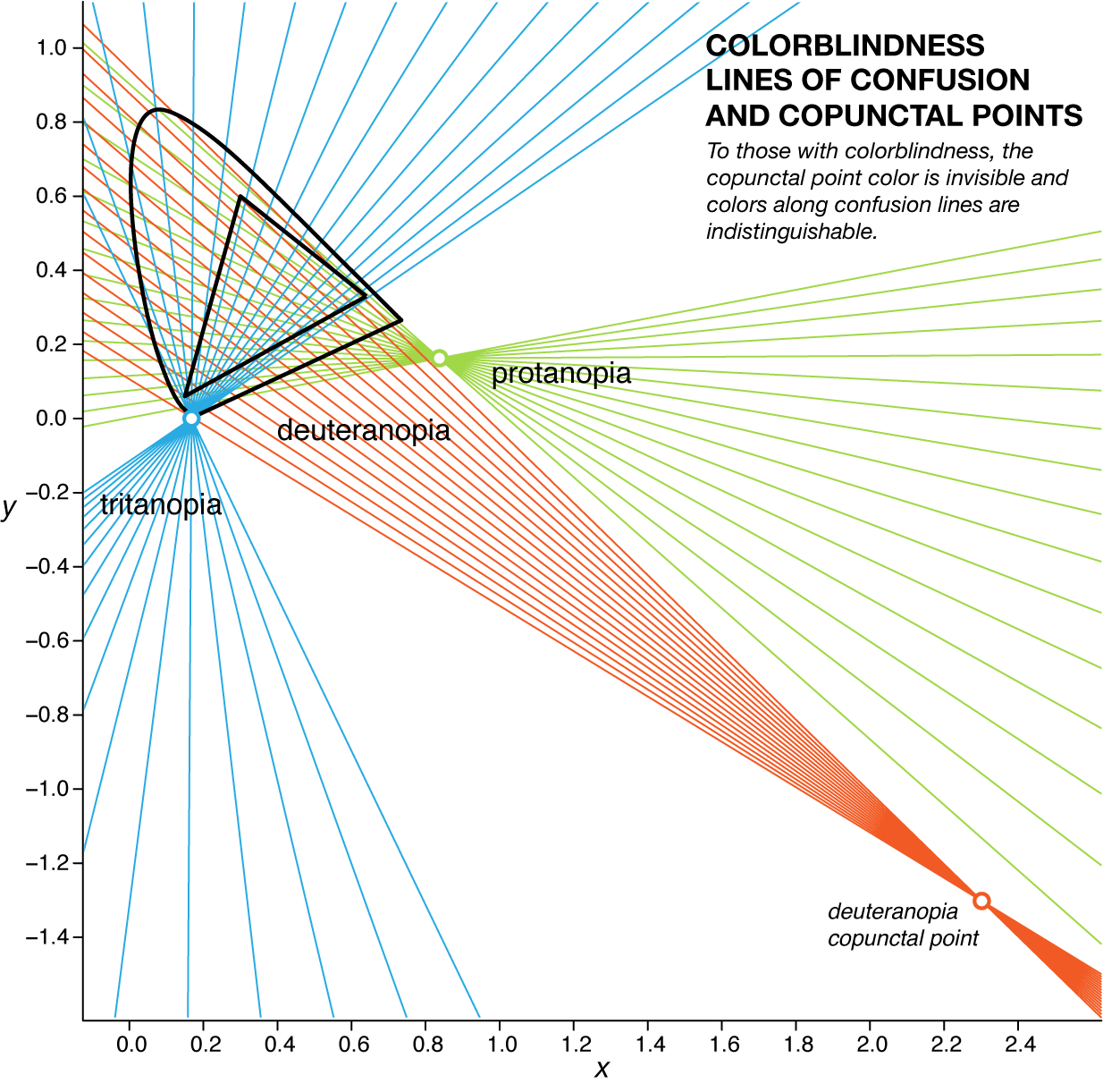
The copunctal point corresponds to the "invisible color" associated with the third eigenvector `\mathbf{v}_{\lambda=0}`. It can be thought of as the colorblind person's third primary color. For trichromats (individuals with normal color vision) there are three primaries. In sRGB space you can think of these as the corners of the triangle that is the sRGB gamut (which primaries you choose doesn't matter, as long as they're not collinear). The primary associated with the missing photoreceptor in dichromats is the copunctal point. We can mix this invisible primary with any other color and not affect how it appears under the colorblind transformation. For a more thorough explanation of this see the section "Köning's concept of the dichromatic copunctal points" in Dichromatic confusion lines and color vision models by G.A. Fry.
The concept of an invisible color is purely a mathematical construct that is helpful in the calculations. Just because it exists outside of the range of human perception (ouside of the CIE monochromatic horseshoe) does not mean it's necessarily theoretically impossible — in many cases, only practially impossible, such as the so-called impossible colors, which are really fun to think about. For example, if the LMS color receptors could be stimulated with an arbitrary ratio of `(L,M,S)` then who knows what would be perceived! For example, the scenario `(L,M,S) = (0,1,0)` is impossible because any wavelength that stimulates M stimulates either S or L. Such a color would have `(X,Y,Z) = (-1.13,0.64,0)` and `(x,y) = (2.3,-1.3)` might appear as "hyper-green" or "beyond-green" Recognize this coordinate? It's the deuteranopia copunctal point — the invisible color for someone who is missing L color receptors!
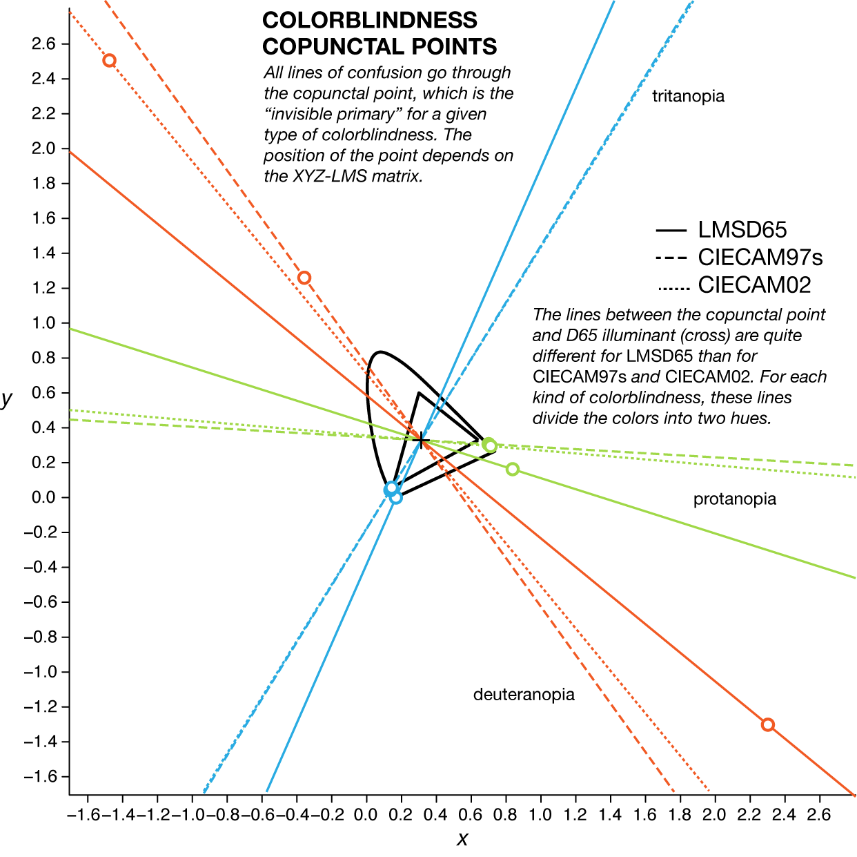
In `XYZ` space, the copunctal points for `\mathbf{M}_{\textrm{LMSD65}}` (the position of these points will depend on what `XYZ` to `LMS` conversion matrix is used) are $$ \mathbf{v}_{XYZ,\textrm{p},\lambda=0} = \left[ \begin{matrix} -0.9816605 \\ -0.1906374 \\ 0 \end{matrix} \right] \qquad \mathbf{v}_{XYZ,\textrm{d},\lambda=0} = \left[ \begin{matrix} -0.8704299 \\ 0.4922923 \\ 0 \end{matrix} \right] \qquad \mathbf{v}_{XYZ,\textrm{t},\lambda=0} = \left[ \begin{matrix} 0.1979166 \\ 0 \\ 0.9802189 \end{matrix} \right] $$
and in `xyY` space they are $$ \mathbf{v}_{xyY,\textrm{p},\lambda=0} = \left[ \begin{matrix} 0.8373814 \\ 0.1626186 \\ 0 \end{matrix} \right] \qquad \mathbf{v}_{xyY,\textrm{d},\lambda=0} = \left[ \begin{matrix} 2.301887 \\ -1.301887 \\ 0 \end{matrix} \right] \qquad \mathbf{v}_{xyY,\textrm{t},\lambda=0} = \left[ \begin{matrix} 0.1679923 \\ 0 \\ 0.8320132 \end{matrix} \right] $$
These eigenvectors can also be calculated directly by transforming the unit vectors in `LMS` space to `XYZ`, since they correspond to the "invisible color" (see discussion above) for each kind of colorblindness. $$ \mathbf{v}_{XYZ,\textrm{p},\lambda=0} = \mathbf{M}^{-1}_{\textrm{LMSD65}} \left[ \begin{matrix} 1 \\ 0 \\ 0 \end{matrix} \right] \qquad \mathbf{v}_{XYZ,\textrm{d},\lambda=0} = \mathbf{M}^{-1}_{\textrm{LMSD65}} \left[ \begin{matrix} 0 \\ 1 \\ 0 \end{matrix} \right] \qquad \mathbf{v}_{XYZ,\textrm{t},\lambda=0} = \mathbf{M}^{-1}_{\textrm{LMSD65}} \left[ \begin{matrix} 0 \\ 0 \\ 1 \end{matrix} \right] $$
The position of the copunctal point depends on which `XYZ` to `LMS` transformation matrix is used (LMSD65, SMSCAM97, LMSCAM02). These matrices represent an approximation of the transformation between `XYZ` and `LMS` spaces. The successor to CIECAM02 is CIECAM16.
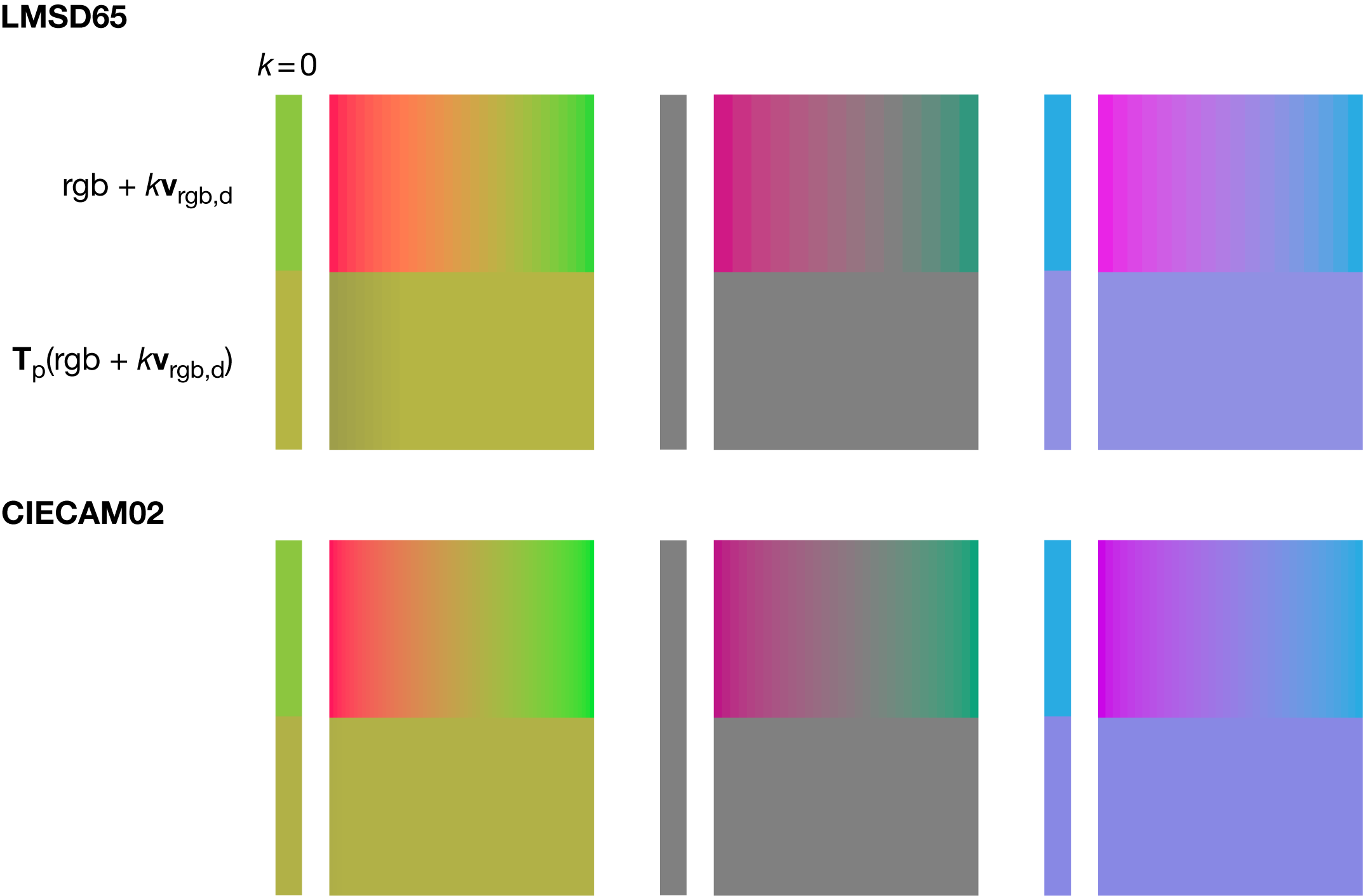
Given an `(R,G,B)` color, to calculate the set of colors along the line of confusion for a given type of colorblindness proceeds as follows. First, linearize the color to `(r,g,b)` (see above) and add any multiple of the `LMS` invisible primary expressed in `rgb` and then convert from linear `rgb` to `RGB`.
For LMSD65, these `rgb` invisible primaries are $$ \mathbf{v}_\textrm{rgb,p} = \left[ \begin{matrix} 5.47221206 \\ -1.12524190 \\ 0.02980165 \end{matrix} \right] \qquad \mathbf{v}_\textrm{rgb,d} = \left[ \begin{matrix} -4.6419601 \\ 2.2931709 \\ -0.1931807 \end{matrix} \right] \qquad \mathbf{v}_\textrm{rgb,t} = \left[ \begin{matrix} 0.1696371 \\ -0.1678952 \\ 1.1636479 \end{matrix} \right] $$
and for CIECAM02 they are $$ \mathbf{v}_\textrm{rgb,p} = \left[ \begin{matrix} 2.8583111 \\ -0.2104348 \\ -0.0418895 \end{matrix} \right] \qquad \mathbf{v}_\textrm{rgb,d} = \left[ \begin{matrix} -1.6287080 \\ 1.1584149 \\ -0.1181543 \end{matrix} \right] \qquad \mathbf{v}_\textrm{rgb,t} = \left[ \begin{matrix} -0.0248186967 \\ 0.0003204633 \\ 1.0688865654 \end{matrix} \right] $$
For example, suppose you want to find all the colors equivalent to `RGB=(140,198,63)` in deuteranopia. First linearize to `rgb=(0.262,0.565,0.0497)`. Then add some multiple of `\mathbf{v}_\textrm{rgb,d}` to get the color `rgb+k\mathbf{v}_\textrm{rgb,d}` and discard any mix that has any negative components. For example, if we use LMSD65 and `k=-0.15` we get a mix `rgb=(0.959,0.221,0.079)` that converts to `RGB=(250,129,78)`. Both this and the original color appear as `RGB=(181,181,68)` to deuteranopes. If instead we used CIECAM02 then all the mixes would appear as `RGB=(177,177,71)`.
Nasa to send our human genome discs to the Moon
We'd like to say a ‘cosmic hello’: mathematics, culture, palaeontology, art and science, and ... human genomes.


Comparing classifier performance with baselines
All animals are equal, but some animals are more equal than others. —George Orwell
This month, we will illustrate the importance of establishing a baseline performance level.
Baselines are typically generated independently for each dataset using very simple models. Their role is to set the minimum level of acceptable performance and help with comparing relative improvements in performance of other models.

Unfortunately, baselines are often overlooked and, in the presence of a class imbalance5, must be established with care.
Megahed, F.M, Chen, Y-J., Jones-Farmer, A., Rigdon, S.E., Krzywinski, M. & Altman, N. (2024) Points of significance: Comparing classifier performance with baselines. Nat. Methods 20.
Happy 2024 π Day—
sunflowers ho!
Celebrate π Day (March 14th) and dig into the digit garden. Let's grow something.

How Analyzing Cosmic Nothing Might Explain Everything
Huge empty areas of the universe called voids could help solve the greatest mysteries in the cosmos.
My graphic accompanying How Analyzing Cosmic Nothing Might Explain Everything in the January 2024 issue of Scientific American depicts the entire Universe in a two-page spread — full of nothing.

The graphic uses the latest data from SDSS 12 and is an update to my Superclusters and Voids poster.
Michael Lemonick (editor) explains on the graphic:
“Regions of relatively empty space called cosmic voids are everywhere in the universe, and scientists believe studying their size, shape and spread across the cosmos could help them understand dark matter, dark energy and other big mysteries.
To use voids in this way, astronomers must map these regions in detail—a project that is just beginning.
Shown here are voids discovered by the Sloan Digital Sky Survey (SDSS), along with a selection of 16 previously named voids. Scientists expect voids to be evenly distributed throughout space—the lack of voids in some regions on the globe simply reflects SDSS’s sky coverage.”
voids
Sofia Contarini, Alice Pisani, Nico Hamaus, Federico Marulli Lauro Moscardini & Marco Baldi (2023) Cosmological Constraints from the BOSS DR12 Void Size Function Astrophysical Journal 953:46.
Nico Hamaus, Alice Pisani, Jin-Ah Choi, Guilhem Lavaux, Benjamin D. Wandelt & Jochen Weller (2020) Journal of Cosmology and Astroparticle Physics 2020:023.
Sloan Digital Sky Survey Data Release 12
Alan MacRobert (Sky & Telescope), Paulina Rowicka/Martin Krzywinski (revisions & Microscopium)
Hoffleit & Warren Jr. (1991) The Bright Star Catalog, 5th Revised Edition (Preliminary Version).
H0 = 67.4 km/(Mpc·s), Ωm = 0.315, Ωv = 0.685. Planck collaboration Planck 2018 results. VI. Cosmological parameters (2018).
constellation figures
stars
cosmology
Error in predictor variables
It is the mark of an educated mind to rest satisfied with the degree of precision that the nature of the subject admits and not to seek exactness where only an approximation is possible. —Aristotle
In regression, the predictors are (typically) assumed to have known values that are measured without error.
Practically, however, predictors are often measured with error. This has a profound (but predictable) effect on the estimates of relationships among variables – the so-called “error in variables” problem.

Error in measuring the predictors is often ignored. In this column, we discuss when ignoring this error is harmless and when it can lead to large bias that can leads us to miss important effects.
Altman, N. & Krzywinski, M. (2024) Points of significance: Error in predictor variables. Nat. Methods 20.
Background reading
Altman, N. & Krzywinski, M. (2015) Points of significance: Simple linear regression. Nat. Methods 12:999–1000.
Lever, J., Krzywinski, M. & Altman, N. (2016) Points of significance: Logistic regression. Nat. Methods 13:541–542 (2016).
Das, K., Krzywinski, M. & Altman, N. (2019) Points of significance: Quantile regression. Nat. Methods 16:451–452.