Learning Circos
Bioinformatics and Genome Analysis
Fondazione Edmund Mach, San Michele all'Adige, Italy, 20 June 2019
v2.00 16 June 2019 Download PDF slides
v2.00 16 June 2019
A 1-day practical course in genomic data visualization with Circos. This material is part of the Bioinformatics and Genome Analysis course held at the Fondazione Edmund Mach in San Michele all'Adige, Italy. Materials also available here: course materials and PDF slides.
Quick links
MyPads | BCGA 2019 | 4-day Circos course | Circos documentation best practices getting started | Brewer palettes | Color resources | Nature Methods Points of View Points of Significance
Genomic Data Visualization with Circos
Thursday 20 June 2019 — Day 1
09h00 – 10h30 | Lecture 1 — Introduction to Circos
11h00 – 12h30 | Lecture (practical) 2 — Visualizing gene distribution and size in Yeast—the histogram data track
14h00 – 15h30 | Lecture (practical) 3 — Conservation in Yeast—the link data track
16h00 – 18h00 | Lecture (practical) 4 — Drawing the human genome
18h15 – 19h30 | Lecture (practical) 5 — Afterhours—Perl refresher
18h15 – 19h30 | Lecture (practical) 6 — Afterhours—Visualizing an Ebola strain
Concepts covered today
Circos configuration, common Circos errors, Circos debugging, ideograms, selecting ideograms with regular expressions, input data format, creating Circos data files, data tracks (histograms, heat map, tiles, links), color definitions and using transparency, Brewer palettes, dynamic data formatting rules, downloading files from UCSC genome browser, essential command-line tools and basic scripting,
Afterhours—Visualizing an Ebola strain
Knowing how to preparing data files efficiently is a very important skill that you must continue to develop.
Let's practise this by creating images of Ebola data downloaded from UCSC genome browser.
Downloading and Parsing Ebola Data
Sometimes your data is already almost nearly in the right format and can be quickly parsed to the format that Circos expects.
Here command-line tools like grep, sed and awk shine and you should become as familiar with them as possible. I cannot stress this enough: a lot of scripting can be entirely avoided by piping calls to these tools.
Let's start with Ebola! I downloaded three tracks for the Sierra Leone Ebola virus assembly, lecture.6/data/ebola.{assembly,genes,variation}.txt, which you can access at
https://genome.ucsc.edu/cgi-bin/hgTables
by selecting "Clade: Viruses" and "Genome: Ebola virus".
 Mapping and sequencing tracks: assembly
 lecture.6/data/ebola.assembly.txt

 Genes and gene prediction tracks: NCBI genes
 lecture.6/data/ebola.genes.txt

 Variation and repeats: 2014 specific
 lecture.6/data/ebola.variation.txt
If we're going to draw any data on the Ebola genome, we need to create the karyotype file that defines the Ebola genome's chromosome. In this case there's only one, so it's trivial to make. You can look at the last line of the data file to see the size of the chromosome
 tail -1 ebola.assembly.txt
 585 KM034562v1 0 18957...
You can make the file by hand by simply creating the file
 # lecture.6/data/ebola.karyotype.txt
 chr - ebola ebola 0 18957 black
or alternatively if you're feeling frisky you can automate this step if you don't want to risk making a mistake entering the length.
 lecture.6/data/make.ebola.karyotype
 tail -1 ebola.assembly.txt | cut -f 4 | awk '{print "chr - ebola ebola 0",$1,"black"}' > ebola.karyotype.txt
Great! You're ready to draw the genome (no data yet).
#!/bin/bash

echo "parsing UCSC assembly table and making karyotype file"
tail -1 ebola.assembly.txt | cut -f 4 | awk '{print "chr - ebola ebola 0",$1,"black"}' > ebola.karyotype.txt
We reference the karyotype file we made in the previous part of this lecture.
chr - ebola ebola 0 18895 black
karyotype = ../data/ebola.karyotype.txt
I have adjusted the thickness of the ideogram to 5 pixels and also the ticks. If you like you can peek into these files.
<<include ../etc/ideogram.conf>>
<<include ../etc/ticks.conf>>
Creating Circos data files for Ebola genes and SNPs
Now that we have the ideogram drawn, let's pull out the gene regions from the gene table file. This file has a pretty simple format. The columns are
bin        585         Indexing field to speed chromosome range queries.
name       NP          Name of gene
chrom      KM034562v1  Reference sequence chromosome or scaffold
strand     +         ) + or - for strand
txStart    55          Transcription start position (or end position for minus strand item)
txEnd      3026        Transcription end position (or start position for minus strand item)
cdsStart   469         Coding region start (or end position for minus strand item)
cdsEnd     2689        Coding region end (or start position for minus strand item)
exonCount  1           Number of exons
exonStarts 55,         Exon start positions (or end positions for minus strand item)
exonEnds   3026,       Exon end positions (or start positions for minus strand item)
This is going to be quick — there are only 9 entries in the gene file! Here I've added a comment row with a row of 1-indexed column for convenience.
# lecture.4/data/ebola.genes.txt
# 1 2    3          4 5     6     7     8     9 10         11
585 NP   KM034562v1 + 55    3026  469   2689  1 55,        3026,
585 VP35 KM034562v1 + 3031  4407  3128  4151  1 3031,      4407,
585 VP40 KM034562v1 + 4389  5894  4478  5459  1 4389,      5894,
585 GP   KM034562v1 + 5899  8305  6038  8068  2 5899,6922, 6920,8305,
585 sGP  KM034562v1 + 5899  8305  6038  7133  1 5899,      8305,
585 ssGP KM034562v1 + 5899  8305  6038  6933  2 5899,6923, 6922,8305,
585 VP30 KM034562v1 + 8287  9740  8508  9375  1 8287,      9740,
585 VP24 KM034562v1 + 9884  11518 10344 11100 1 9884,      11518,
585 L    KM034562v1 + 11500 18282 11580 18219 1 11500,     18282,
It's up to us what to draw. Let's pull out the gene start and end positions, its name and the number of exons. We'll pull out column 2, 5, 6 and 9 using cut (remember cut starts indexing at 1 not zero) and then rearrange them with awk, since cut doesn't offer the option for changing column order.
#lecture.6/data/create.ebola.tracks
grep -v ebola.genes.txt | cut -f 2,5,6,9 | awk '{print "ebola",$2,$3,$4,"name="$1}' > track.ebola.genes.txt
This gives us this file
# lecture.6/data/track.ebola.genes.txt
ebola 55 3026 1 name=NP
ebola 3031 4407 1 name=VP35
ebola 4389 5894 1 name=VP40
ebola 5899 8305 2 name=GP
ebola 5899 8305 1 name=sGP
ebola 5899 8305 2 name=ssGP
ebola 8287 9740 1 name=VP30
ebola 9884 11518 1 name=VP24
ebola 11500 18282 1 name=L
Next, let's parse the variations, which are SNPs. The variationfile has the following tab-delimited fields
chrom      KM034562v1 Reference sequence
chromStart 8985       Start position in reference
chromEnd   8986       End position in reference
name       A/C        Variant: ancestral/2014-derived
score      0          Score from 0-1000 (not used)
strand     +          + or - (always + here)
thickStart 8985       Start of where display should be thick (same as chromStart)
thickEnd   8986       End of where display should be thick (same as chromEnd)
reserved   0,220,0    Used as itemRgb
gene       VP30       Gene symbol
type       synonymous noncoding, synonymous or nonsynonymous
hgsv       VP30:Arg160Arg HGSV notation for protein coding changes (or lack thereof)
blosum62   NA             BLOSUM62 substitution score for ancestral and 2014 amino acids
countInNew 81             Number of 2014 samples that contain derived allele (out of 81 total)
freqInNew  1.000000       Derived allele frequency of 2014 samples
and the first few lines are
# lecture.6/data/ebola.variation.txt
#  1       2   3   4   5 6 7   8   9     10 11         12 13 14
KM034562v1 126 127 C/T 0 + 126 127 0,0,0 NP noncoding  NA 81 1.000000
KM034562v1 154 155 A/C 0 + 154 155 0,0,0 NP noncoding  NA 81 1.000000
KM034562v1 181 182 A/G 0 + 181 182 0,0,0 NP noncoding  NA 81 1.000000
KM034562v1 186 187 A/G 0 + 186 187 0,0,0 NP noncoding  NA 81 1.000000
...
I've added a comment row with a row of zero-indexed column for convenience.
# lecture.6/data/create.ebola.tracks
grep -v ebola.variation.txt | cut -f 2,3,4,10,15 | \
  perl -pe 's/\w+:\w+//' | \
  awk '{print "ebola",$2,$3,$5,"snp="$1",gene="$4}' > track.ebola.variation.txt
gives us
#lecture.6/data/track.ebola.variation.txt
ebola 126 127 1.000000 snp=C/T,gene=NP
ebola 154 155 1.000000 snp=A/C,gene=NP
ebola 181 182 1.000000 snp=A/G,gene=NP
ebola 186 187 1.000000 snp=A/G,gene=NP
...
#!/bin/bash

# extract genes

echo "Creating gene track"
grep -v \# ebola.genes.txt | cut -f 2,5,6,9 | \
    awk '{print "ebola",$2,$3,$4,"name="$1}' > track.ebola.genes.txt

# extract SNPs

echo "Creating SNP track"
grep -v \# ebola.variation.txt | cut -f 2,3,4,10,15 | \
    perl -pe 's/\w+:\w+//' | \
    awk '{print "ebola",$1,$2,$5,"snp="$3",gene="$4}' > track.ebola.variation.txt
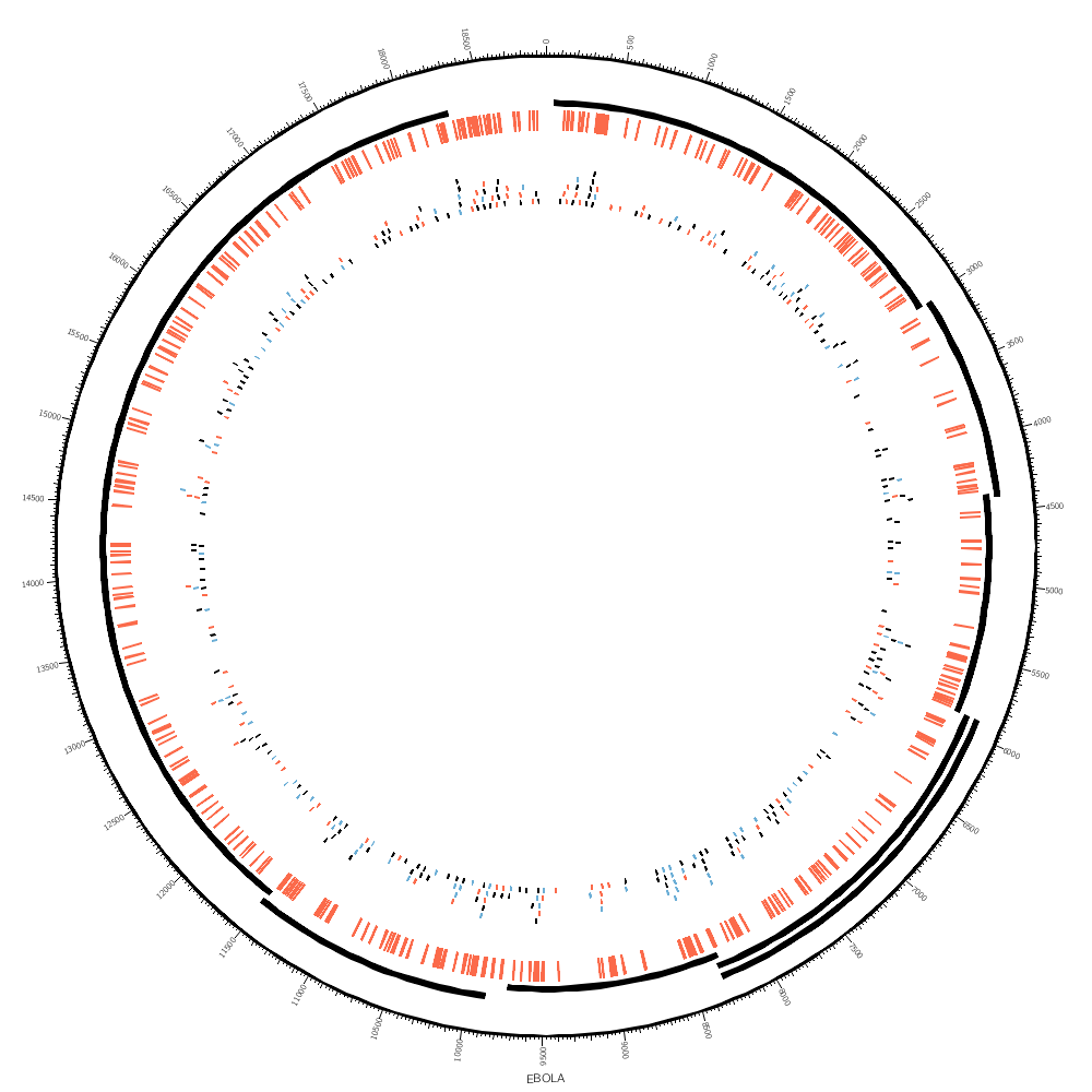
We are now ready to draw the genes and SNPs.
karyotype = ../data/ebola.karyotype.txt

<plots>
We'll draw the gene regions as a tile track. This track automatically organizes regions into layers in a way that avoids overlap. The reason that we need this track is because some of the gene regions overlap.
<plot>
type = tile
file = ../data/track.ebola.genes.txt
r1   = 0.95r
r0   = 0.90r
stroke_thickness = 0
color     = black
margin    = 100u
thickness = 5p
padding   = 5p
</plot>
For the SNPs we can use a highlight track. This track colors the regions defined in the file.
How can we check that all the SNP positions are unique? Make a call to cut, extract the start position, sort it (which is needed for the next step) and report the number of runs of identical values. Finally, grep out any line that doesn't have a "1" applied to matching whole words (i.e. we need the number 1 not just the digit 1 embedded in another number).
cat ../data/track.ebola.variation.txt | cut -d " " -f 2 | sort | uniq -c | grep -v -w 1
Since this command reports no lines, we know that they're uniq. Another way of doing it is counting all lines and unique start values
> wc ../data/track.ebola.variation.txt
395
> cat ../data/track.ebola.variation.txt | cut -d " " -f 2 | sort | uniq | wc
395
Since both commands give us the same count, all start positions are unique.
<plot>
type = highlight
file = ../data/track.ebola.variation.txt
fill_color = red
stroke_thickness = 0
r1   = 0.89r
r0   = 0.85r
Since the SNP regions are a single base in size, they're small and hard to see. In these cases you can use minsize to expand the size of the data point to be at least this minimum size. Beware that this changes how people might interpret the data — but it's better to be able to see the data clearly than not.
minsize = 10

</plot>
It's worth exploring how the SNPs might look when drawn as tiles. Each tile is a single SNP, enlarged here so that you can see it more clearly. It's now very obvious where SNPs are close together — something that we couldn't see with the highlight track above.
<plot>
type = tile
file = ../data/track.ebola.variation.txt

r1   = 0.79r
r0   = 0.70r
You can make the size larger (try 25). Below 10 it's impossible to see the SNPs. That is because the genome is about 14 kb in size and the circumference of the circle is about 3,000 pixels. Thus, a single base is only 1/5th of a pixel!
minsize = 10

stroke_thickness = 0
color     = black
This is how close SNPs can be to one another in the same layer.
margin    = 20u
thickness = 4p
padding   = 3p

layers_overflow = grow

<rules>

<rule>
condition = var(snp) =~ /^A/
color     = red
</rule>

<rule>
condition = var(snp) =~ /A$/
color     = blue
</rule>

</rules>

</plot>

</plots>
Edit lecture.6/data/create.ebola.tracks to include the type (e.g. noncoding, synonymous, etc) in the data file. How many different types are there? Edit the rules to assign a different color to each type.