
Learning Circos
Bioinformatics and Genome Analysis
Fondazione Edmund Mach, San Michele all'Adige, Italy, 20 June 2019
v2.00 16 June 2019 Download PDF slides
v2.00 16 June 2019
A 1-day practical course in genomic data visualization with Circos. This material is part of the Bioinformatics and Genome Analysis course held at the Fondazione Edmund Mach in San Michele all'Adige, Italy. Materials also available here: course materials and PDF slides.
Quick links
MyPads | BCGA 2019 | 4-day Circos course | Circos documentation best practices getting started | Brewer palettes | Color resources | Nature Methods Points of View Points of Significance
Genomic Data Visualization with Circos
Thursday 20 June 2019 — Day 1
09h00 – 10h30 | Lecture 1 — Introduction to Circos
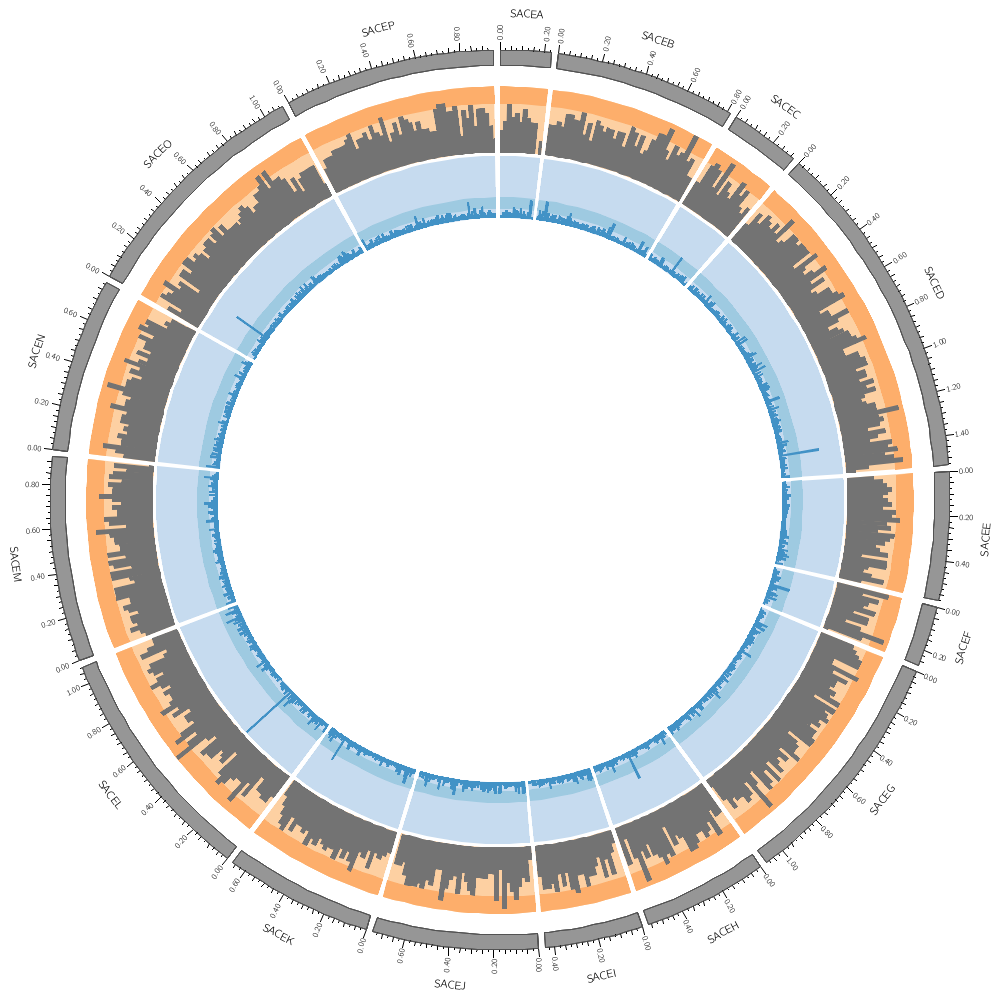
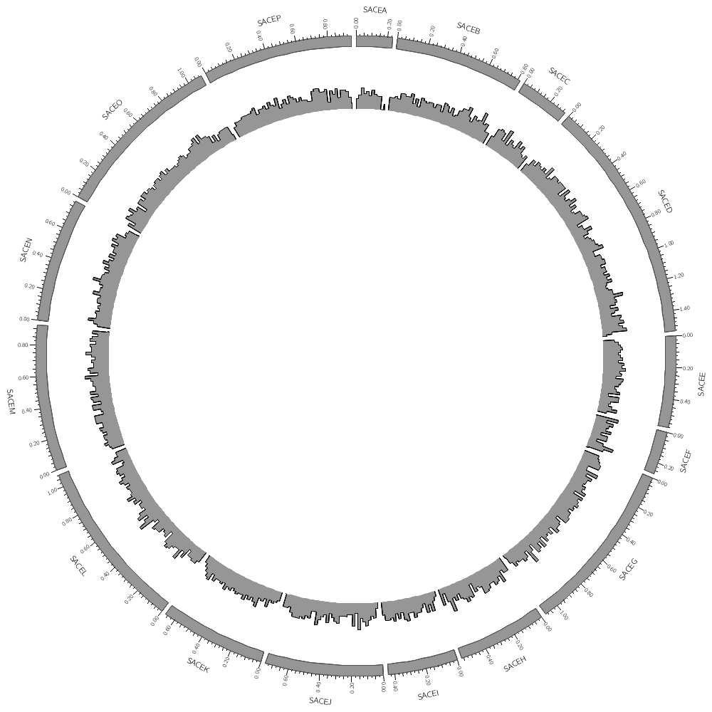
11h00 – 12h30 | Lecture (practical) 2 — Visualizing gene distribution and size in Yeast—the histogram data track
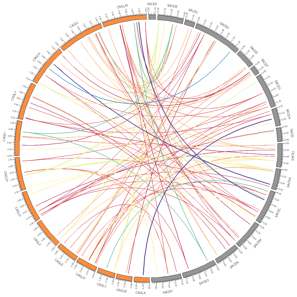
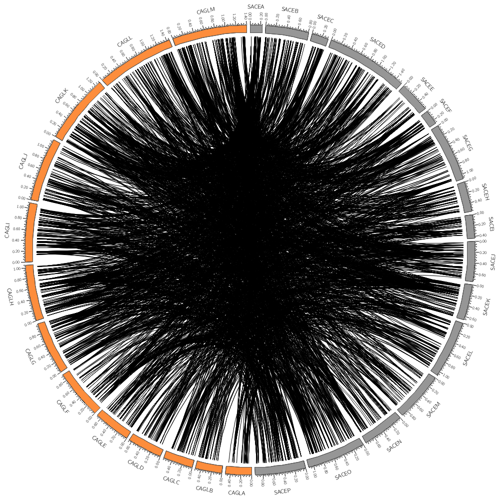
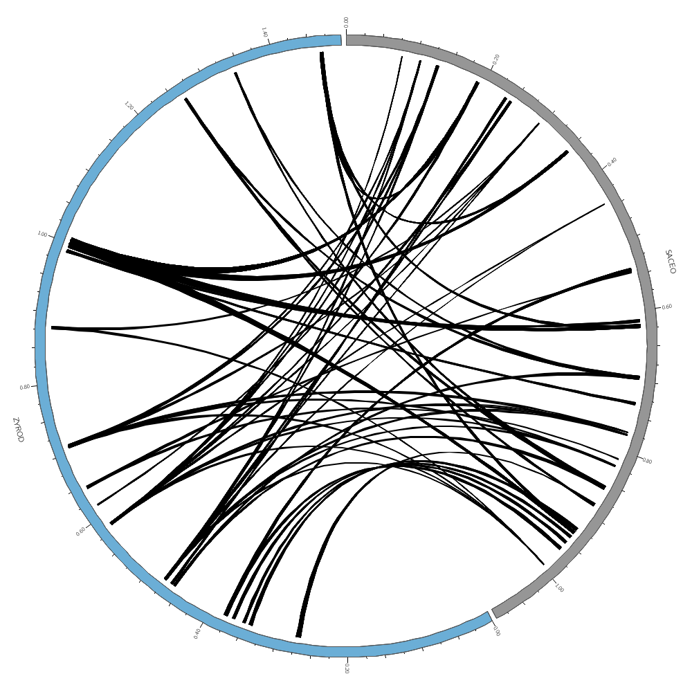
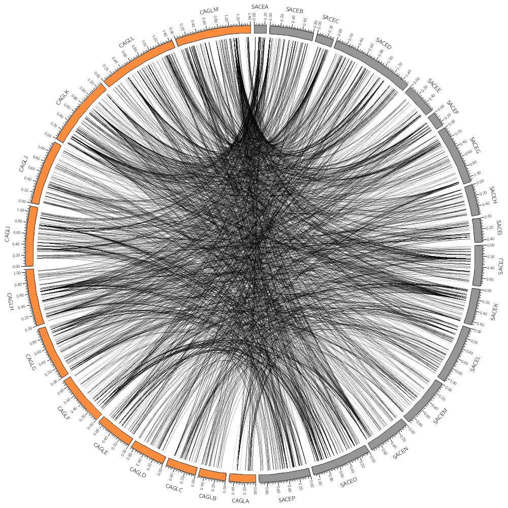
14h00 – 15h30 | Lecture (practical) 3 — Conservation in Yeast—the link data track
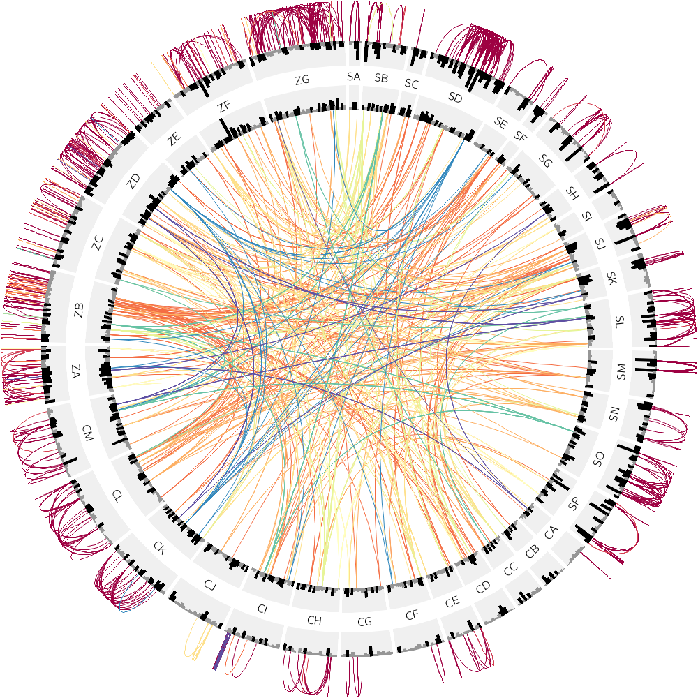
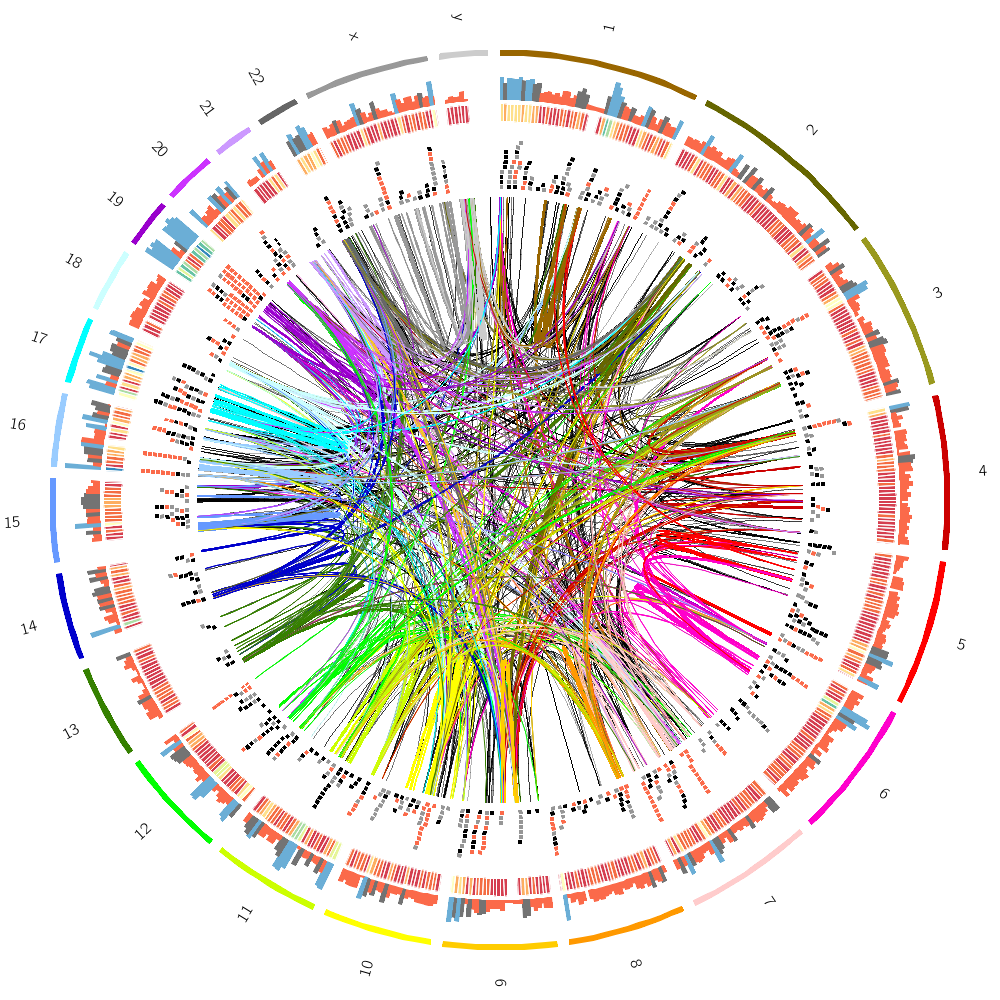
16h00 – 18h00 | Lecture (practical) 4 — Drawing the human genome
18h15 – 19h30 | Lecture (practical) 5 — Afterhours—Perl refresher
18h15 – 19h30 | Lecture (practical) 6 — Afterhours—Visualizing an Ebola strain
Concepts covered today
Circos configuration, common Circos errors, Circos debugging, ideograms, selecting ideograms with regular expressions, input data format, creating Circos data files, data tracks (histograms, heat map, tiles, links), color definitions and using transparency, Brewer palettes, dynamic data formatting rules, downloading files from UCSC genome browser, essential command-line tools and basic scripting,
Introduction to Circos
This lecture covers the file organization of this 1-day course, how to use the files and some commonly seen error messages generated by Circos that you might encounter on the way.
To create the images included in the lectures, you'll need Circos installed.
http://www.circos.ca/documentation/tutorials/configuration/
Today, you will...
 1. learn how Circos works
 2. learn how to visualize a variety of data with Circos
 3. reinforce your command line skills
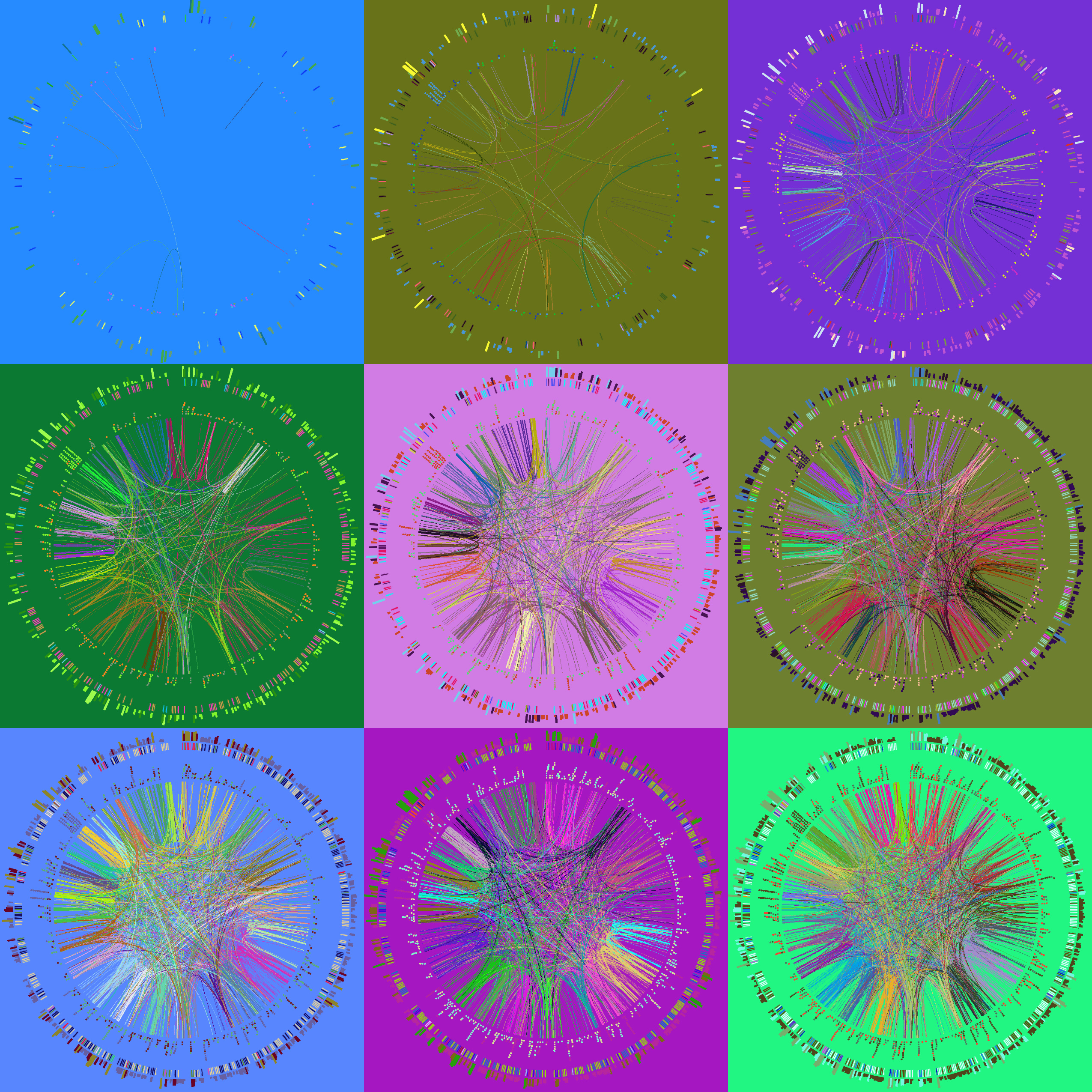
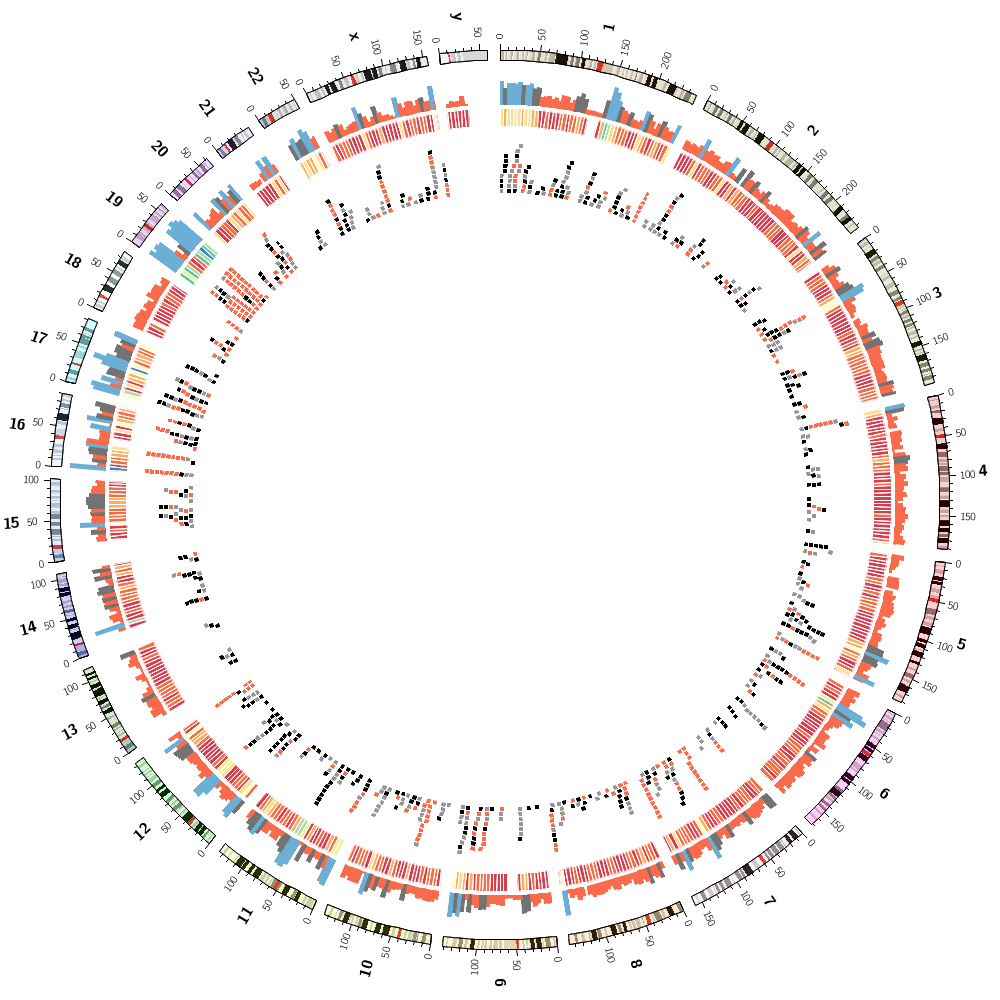
Finally, you will create a unique image montage as a souvenir image to finish off the course!
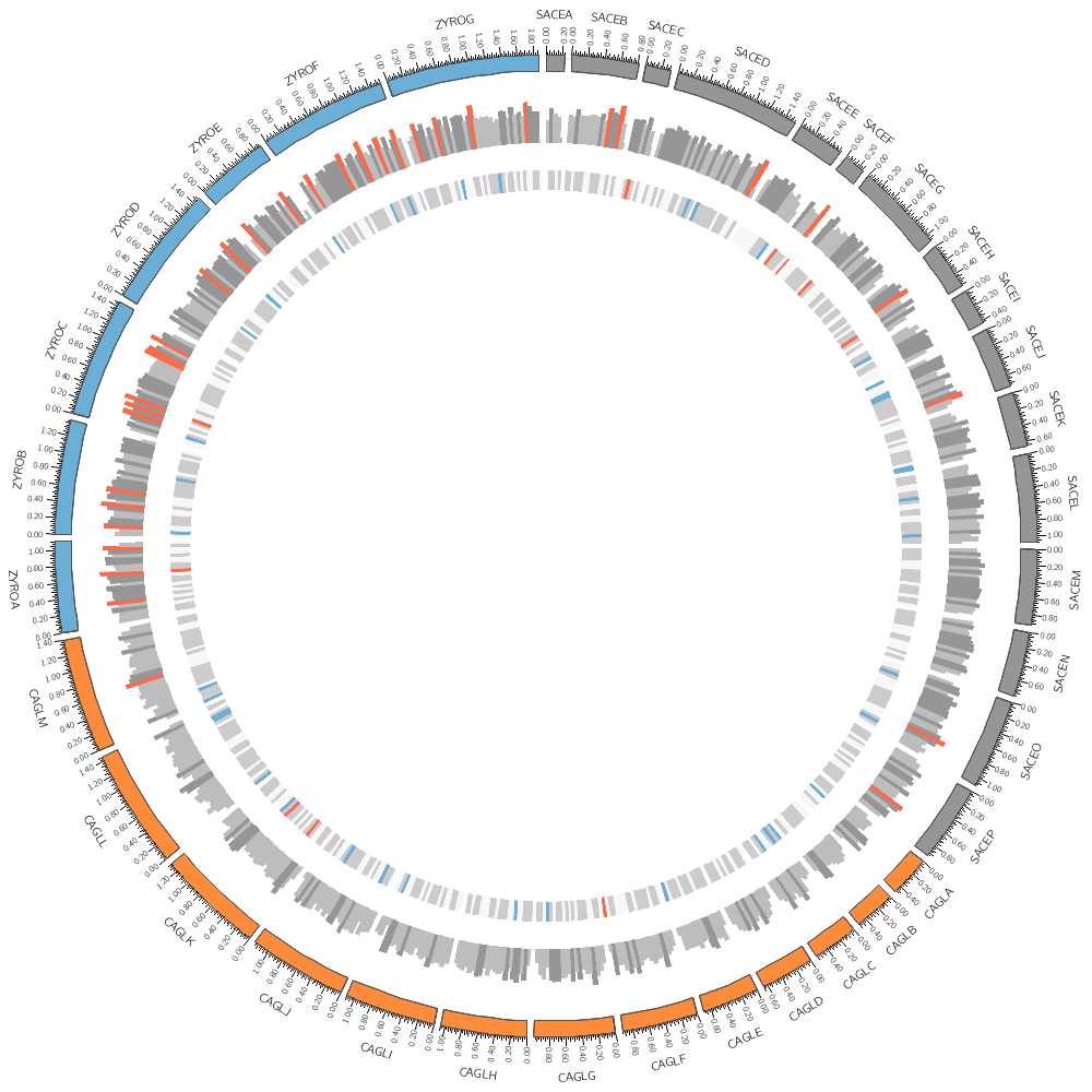
Below are some of the images you'll be creating today.
How Circos works
Circos does not have an interface.
Circos is a command line program.
Circos takes plain-text files as input, which define all aspects of the image.
Circos configuration
A very basic configuration file looks like this
karyotype = ../../data/karyotype.txt

Everything below is details that we'll worry about later.

chromosomes_units = 100
<<include ideogram.conf>>
<<include ../../../etc/ticks.conf>>
<<include ../../../etc/image.conf>>
<<include etc/colors_fonts_patterns.conf>>
<<include etc/housekeeping.conf>>
It is a plain-text file that has a blocks (e.g. <plots>...</plots>) and can <<include ...>> content from other files.
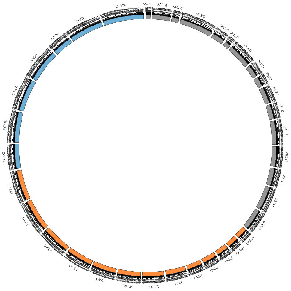
The karyotype.txt file defines the name and length of all the segments placed around the circle.
For example, you'll start off by drawing some data on three different Yeast species, for which the karyotype file is
# chr - name label 0 length color
chr - sace-a saceA 0 230218 grey
chr - sace-b saceB 0 813184 grey
chr - sace-d saceD 0 1531933 grey
...
chr - cagl-a caglA 0 491328 orange
chr - cagl-b caglB 0 502101 orange
chr - cagl-c caglC 0 558804 orange
...
chr - zyro-a zyroA 0 1114666 blue
chr - zyro-b zyroB 0 1388208 blue
chr - zyro-c zyroC 0 1464093 blue
...
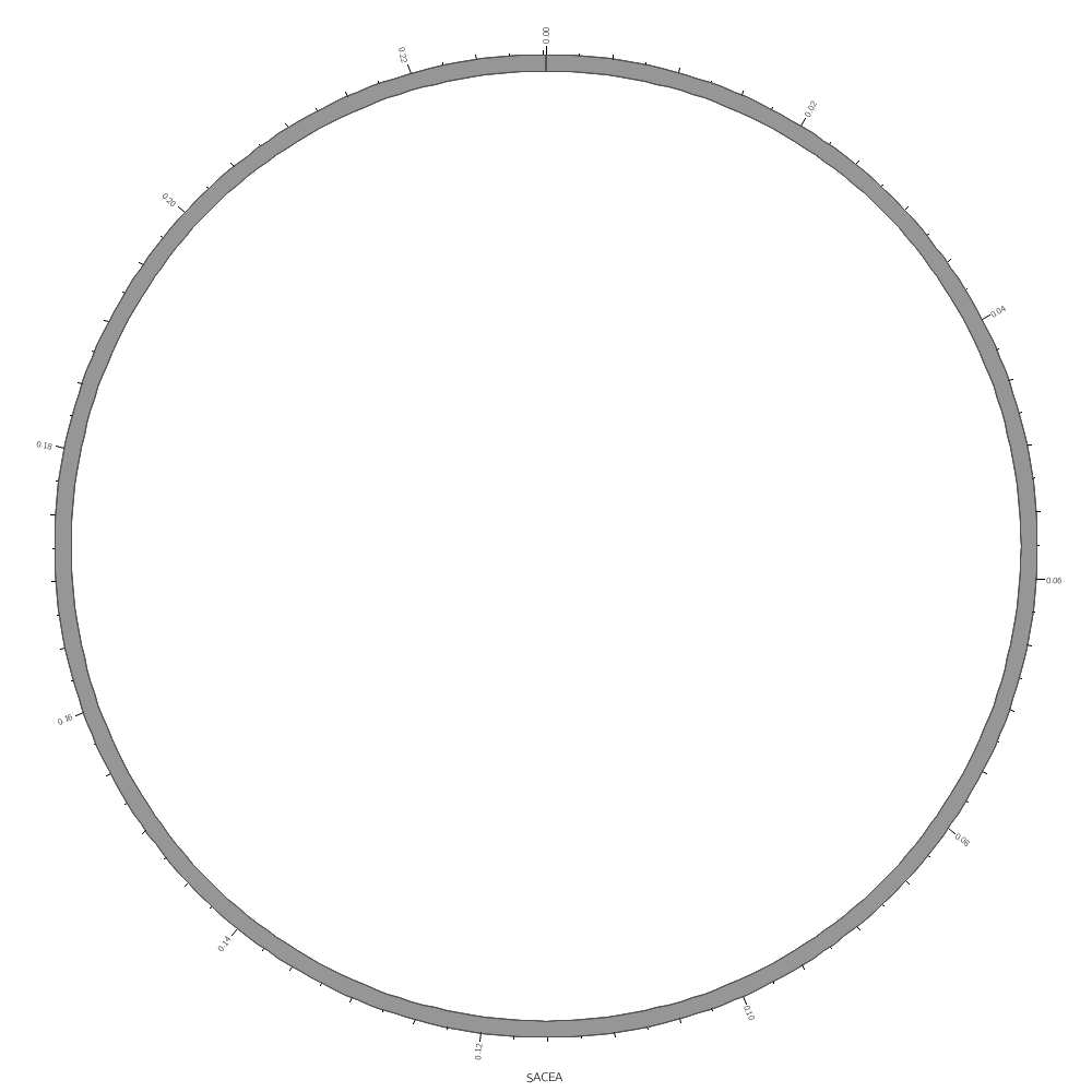
You don't have to draw all the segments defined in the file. For example, by using the chromosomes parameter you can choose to draw only one segment.
chromosomes = sace-a
To draw data segments, you first create a plain-text file
cagl-a 0 19999 1
cagl-a 20000 39999 10
cagl-a 40000 59999 5
...
and then ask Circos to draw the data using <plot> blocks.
<plots>
<plot>
file = ../../data/genes.count.20kb.txt
type = histogram
</plot>
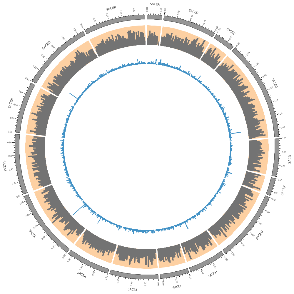
You can add as many plot tracks as you like — they can be placed anywhere in the image. They can even overlap.
To do this, just add another plot block.
<plots>

<plot>
file = ../../data/genes.count.20kb.txt
type = histogram
r1   = 0.95r
r0   = 0.80r
<backgrounds>
<background>
color = vlorange
</background>
</backgrounds>
</plot>

<plot>
file = ../../data/genes.avgsize.10kb.txt
type = histogram
r1   = 0.79r
r0   = 0.65r
fill_color = dblue
</plot>

</plots>
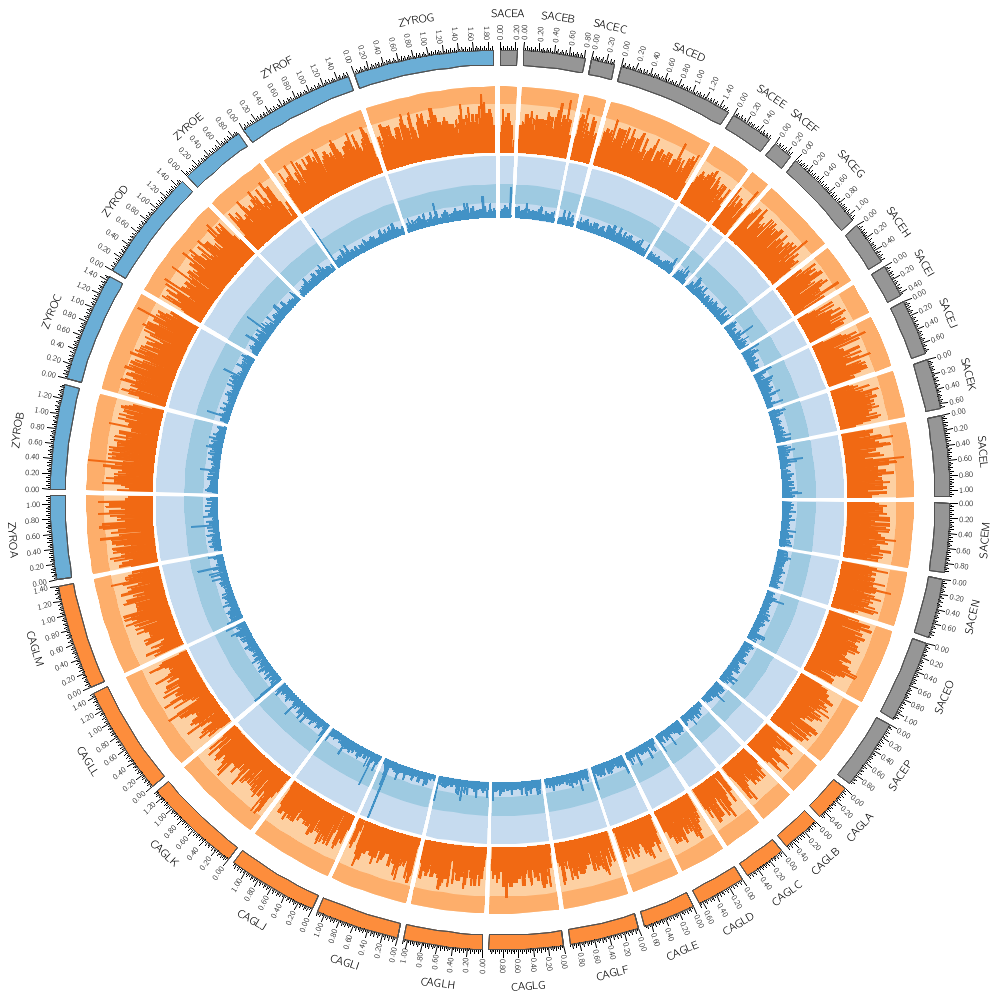
Data sampling
You will then explore how the resolution of data sampling impacts the figure and how to avoid reusing the same color for different encodings.
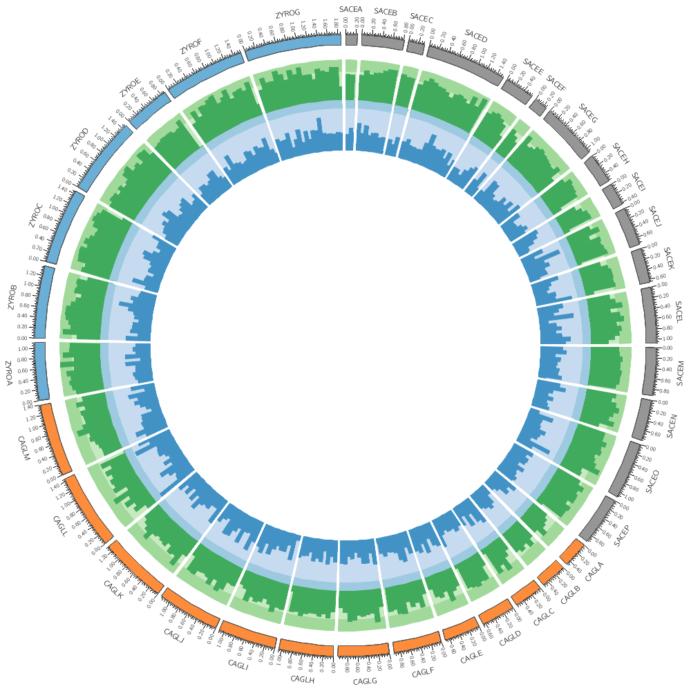
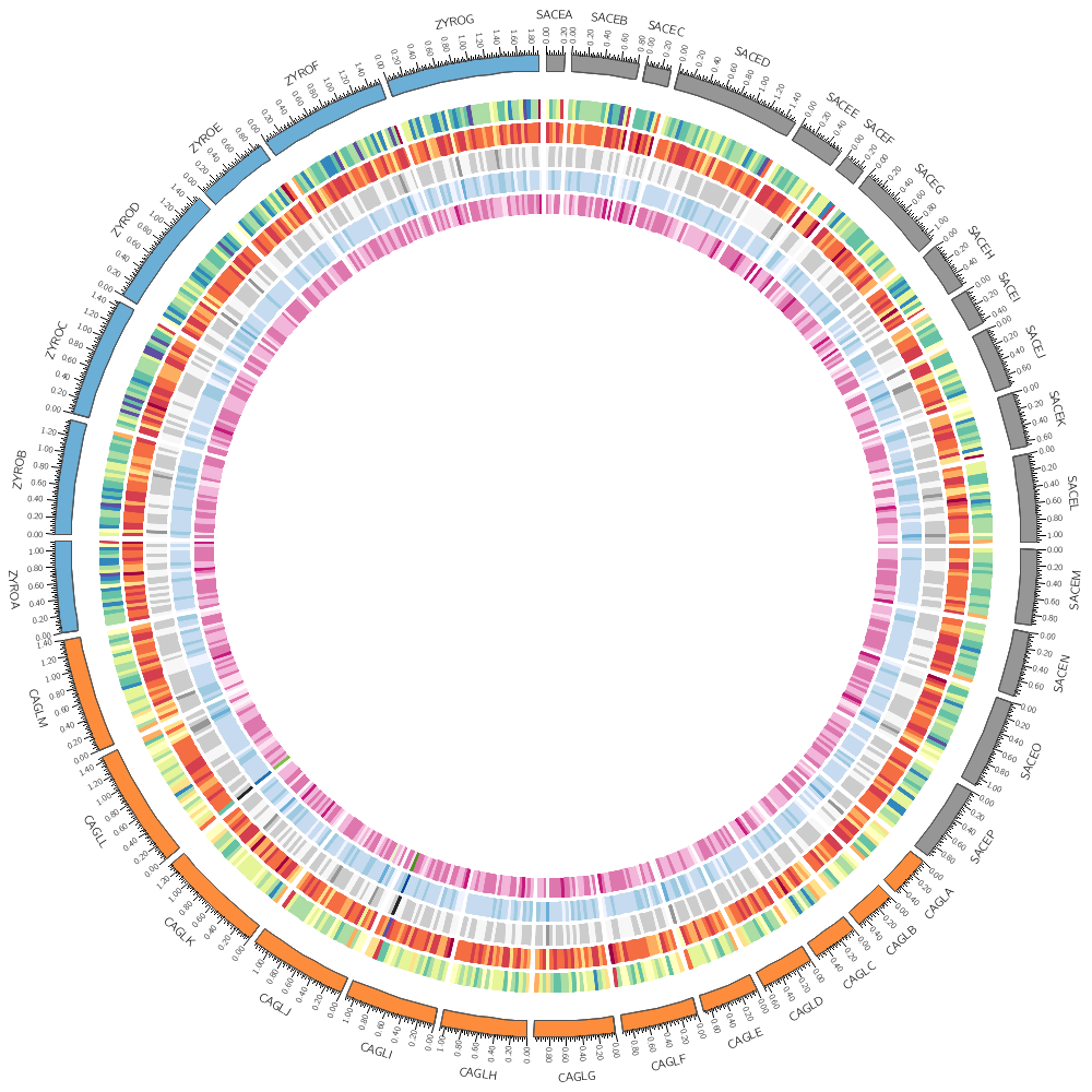
Heat maps
You'll next see how to change histograms to heatmaps and how to use various color schemes.
Brewer colors
Brewer palettes are predefined perceptually uniform color schemes for encoding quantitative and qualitative data.
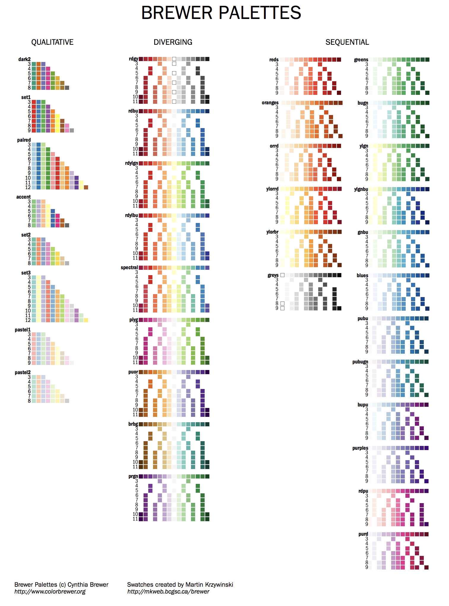
You can find all the swatches for the palette in handouts/brewer-palettes-swatches.pdf or on my Brewer palette resource page.
Color definitions
Each of the k=1..N colors for the N-color palette is defined as
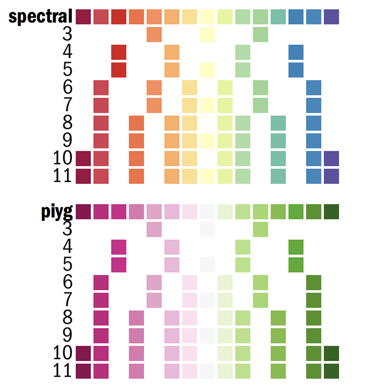
 spectral-N-div-k
 piyg-N-div-k
For example spectral-5-div-1 is the first color (dark red) in the 5-color spectral palette.
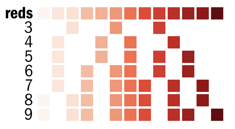
The individual color definitions for red mentioned above are actually based on the Brewer palettes.
vvlred  = reds-7-seq-1
vlred   = reds-7-seq-2
lred    = reds-7-seq-3
red     = reds-7-seq-4
dred    = reds-7-seq-5
vdred   = reds-7-seq-6
vvdred  = reds-7-seq-7
Color encodings
Color is a very useful way to encode information about data.
Circos supports very flexible color definitions.
There are many helpful color names already defined, like
black
grey
red
orange
yellow
blue
green
purple
Each color has a light and dark variant
vvdred    very very dark red
 vdred         very dark red
  dred              dark red
   red                   red
  lred             light red
 vlred        very light red
vvlred   very very light red
Pretty funny, eh?
Dynamic rules
Circos allows you to write simple rules to determine whether and how data should be drawn. These can apply to <plot> and <link> blocks.
<plot>

...

<rules>

<rule>
condition  = var(value) < 50
show       = no
</rule>

<rule>
condition  = var(value) > 250
fill_color = red
</rule>

<rule>
#... another rule
</rule>

</rules>

</link>
Each rule has a condition. Every data point is tested and if the condition is true, the rule applies to the data point and no more rules are tested for that data point (unless you specifically specify that they shoudl). If the condition is not true, subsequent rules are tested.
The rules reference the values and formatting of a data point using var(X) where X is a property like chr, start, end, color and so on.
parsing data on the command line
You're also going to be spending a lot of time on the command line parsing data, asking statistical questions and preparing Circos input files.
 cat - listing a file
grep - matching lines with regular expressions
 sed - replacing strings
 cut - pulling out fields
sort - sorting lines
uniq - counting unique lines
 awk - robust data extraction and reporting tool, particularly useful for rearranging fields
Command line parsing patterns
 List lines from file.txt with top 10 largest values in column 3
> awk '{print $3,$0}' file.txt | sort -nr | head -10 | cut -d " " -f 2-
 List all lines that match neither "abc" nor "def" and replace all instances of "chr" with "hs"
> grep -v 'abc\|def' file.txt | sed 's/chr/hs/g'
 List all lines except comment or blank lines
> egrep -v '^($|#)' file.txt
Circos tools
Circos also comes with helper scripts that achieve common tasks.
Because Circos does not perform analysis (or calculations) you will need to generate data sets sampled at the right resolution.
For example, the resample tool aggregates data in bins and reports statistics like average, min, max and count.
So you can take a list of gene positions and their sizes and create a count of genes in each 10kb window.
sace-a 1807 2169 363 name=YAL068C
sace-a 2480 2707 228 name=YAL067W-A
sace-a 7235 9016 1782 name=YAL067C
sace-a 11565 11951 387 name=YAL065C
sace-a 12046 12426 381 name=YAL064W-B
sace-a 13363 13743 381 name=YAL064C-A
sace-a 21566 21850 285 name=YAL064W
sace-a 22395 22685 291 name=YAL063C-A
...
 cat genes.txt | $DIR/resample/bin/resample -bin 10000 -count
sace-a 0 9999 3
sace-a 10000 19999 3
sace-a 20000 29999 3
...
You can script this to generate counts (and other statistics) for various windows.
for binkb in 50 75 100 ; do
  binsize=$((1000*binkb))
  cat ../../data/genes.txt | $CTOOLS/resample/bin/resample -bin $binsize -count > genes.count.${binkb}kb.txt
  cat ../../data/genes.txt | $CTOOLS/resample/bin/resample -bin $binsize -avg   > genes.avgsize.${binkb}kb.txt
done
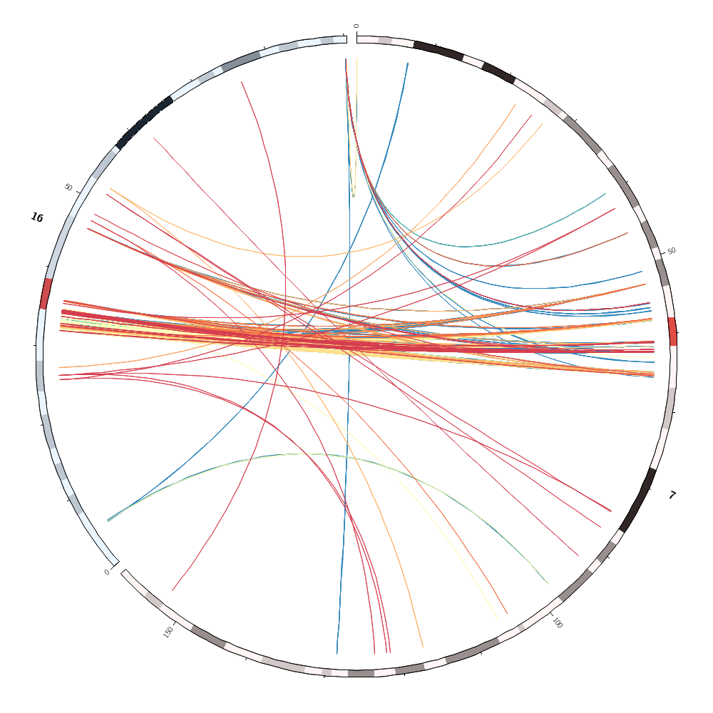
Drawing links
In today's Lecture 3 you will learn how to draw links.
These can represent any relationship between genome positions, such as conservation.
The format of a link file is simple: a pair of coordinates.
cagl-a  19487 21757 sace-g  450197 452104
cagl-a  22260 24440 sace-g  452404 454560
cagl-a  25241 27622 sace-b  207194 209224
...
And links are defined in circos.conf using a <link> block.
<links>
<link>
file = ../../data/links.conservation.10000.txt
radius = 0.98r
...
</link>
</links>
Analyzing distributions
We'll look at how you can quickly analyze distributions of quantities in the data files.
> cat ../../data/links.conservation.txt | awk '{print $3-$2+1}' | ./histogram -min 0 -max 5000 -bin 250
               0.0000>     0  0.000
    0.0000   250.0000    197  0.002  0.002
  250.0000   500.0000   3119  0.030  0.032 *****
  500.0000   750.0000   6557  0.063  0.095 ************
  750.0000  1000.0000   9606  0.093  0.188 ******************
 1000.0000  1250.0000  12679  0.122  0.310 ************************
 1250.0000  1500.0000  11844  0.114  0.425 **********************
 1500.0000  1750.0000  13019  0.126  0.550 *************************
 1750.0000  2000.0000   9172  0.089  0.639 *****************
 2000.0000  2250.0000   6685  0.065  0.703 ************
 2250.0000  2500.0000   7831  0.076  0.779 ***************
 2500.0000  2750.0000   5411  0.052  0.831 **********
 2750.0000  3000.0000   3809  0.037  0.868 *******
 3000.0000  3250.0000   3026  0.029  0.897 *****
 3250.0000  3500.0000   2743  0.026  0.924 *****
 3500.0000  3750.0000   1877  0.018  0.942 ***
 3750.0000  4000.0000   1131  0.011  0.953 **
 4000.0000  4250.0000    893  0.009  0.961 *
 4250.0000  4500.0000   1587  0.015  0.977 ***
 4500.0000  4750.0000   1427  0.014  0.990 **
 4750.0000  5000.0000   1004  0.010  1.000 *
            5000.0000<  1646  0.016
Filtering links
You'll see how rules can be used to filter links and change how they are formatted.
<rules>

<rule>
condition = var(size1) < 5000 || var(size2) < 5000
show      = no
</rule>

<rule>
condition = 1
thickness = eval(sprintf("%d",remap_int(var(size1),5000,10000,1,3)))
z         = eval(var(size1))

</rule>

</rules>
For links, because they are a pair of coordinates, we have chr1, start1 and end1 for the first coordinate and chr2, start2 and end2 for the second.
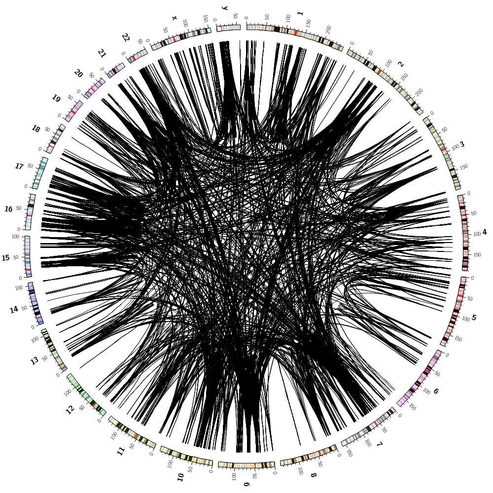
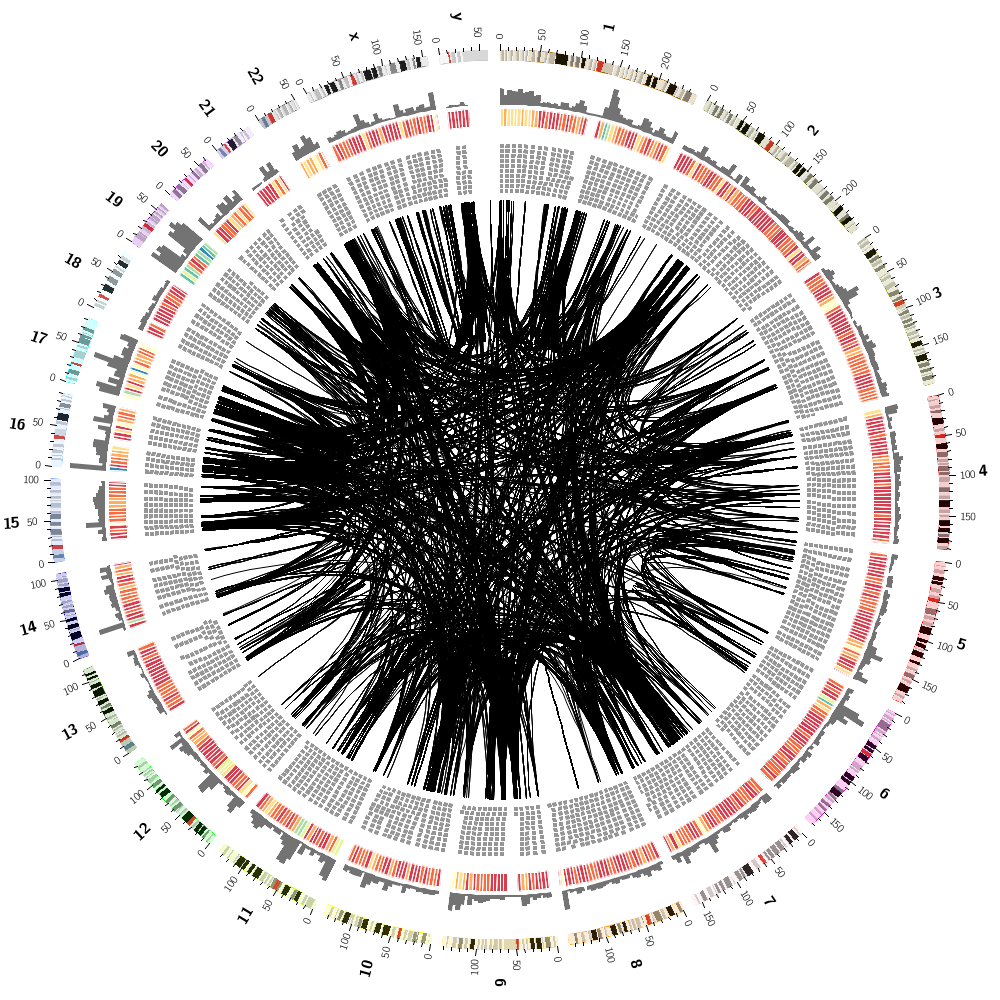
Drawing the human genome
In the last lecture of today, you'll be drawing human genome data: gene positions and segmental duplication.
You have already seen how to draw data: histograms, tiles, links and so on. It's even more important that you are comfortable with parsing and formatting data files.
Human karyotype
Circos comes with karyotype files for organisms like human, rat, mouse and so con.
data/karyotype.human.txt
chr - hs1 1 0 249250621 chr1
chr - hs2 2 0 243199373 chr2
chr - hs3 3 0 198022430 chr3
chr - hs4 4 0 191154276 chr4
chr - hs5 5 0 180915260 chr5
chr - hs6 6 0 171115067 chr6
...
Drawing human genes
Using a list of 61,565 human genes (from UCSC genome browser) you will create a smaller list of about 3,500 genes.
hs19 58346805 58353499 8 name=A1BG
hs10 50799408 50885675 15 name=A1CF
hs12 9067707 9115962 36 name=A2M
hs12 8822471 8876783 36 name=A2ML1
hs1 33306765 33321098 5 name=A3GALT2
...
You will create distributions of gene and segmental duplication sizes with a handy histogram script.
               0.0000>     0  0.000
    0.0000    10.0000   5883  0.324  0.324 *************************
   10.0000    20.0000   3234  0.178  0.503 *************
   20.0000    30.0000   2093  0.115  0.618 ********
   30.0000    40.0000   1428  0.079  0.697 ******
   40.0000    50.0000   1070  0.059  0.756 ****
   50.0000    60.0000    800  0.044  0.800 ***
   60.0000    70.0000    635  0.035  0.835 **
   70.0000    80.0000    471  0.026  0.861 **
   80.0000    90.0000    439  0.024  0.885 *
   90.0000   100.0000    312  0.017  0.902 *
  100.0000   110.0000    334  0.018  0.921 *
  110.0000   120.0000    239  0.013  0.934 *
  120.0000   130.0000    234  0.013  0.947
  130.0000   140.0000    211  0.012  0.959
  140.0000   150.0000    178  0.010  0.968
  150.0000   160.0000    162  0.009  0.977
  160.0000   170.0000    110  0.006  0.983
  170.0000   180.0000    118  0.007  0.990
  180.0000   190.0000     87  0.005  0.995
  190.0000   200.0000     97  0.005  1.000
             200.0000<  1136  0.059
       n        19271
 average     57.84419
      sd    114.60633
     min      0.14800
     max   2304.64000
     sum 1114715.37900
You will then use rules to select which gene families to draw and how to color them. For example
<rule>
condition = var(name) =~ /^ZNF/
color     = red
</rule>

<rule>
condition = 1
show      = no
</rule>
would color red all genes whose name starts with ZNF and hide all others.
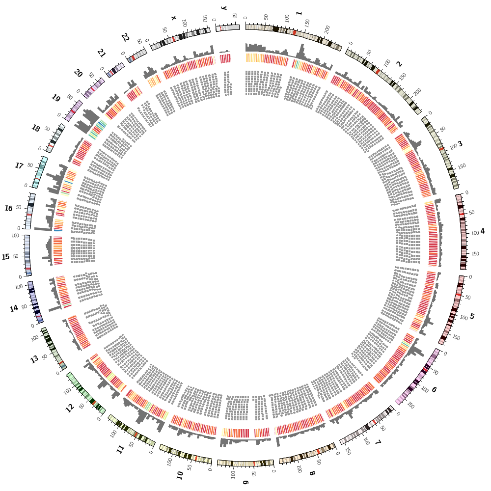
Drawing segmental duplications
You'll create a file in the right format for Circos to draw links, but also with size ranks for each chromosome.
hs1  146541435  146905930  hs16  70811383  71168670 sizerank=1
hs1  148600078  148935345  hs1  119989247  120323081 sizerank=2
hs1  119989247  120323081  hs1  148600078  148935345 sizerank=3
...
hs2  110276210  110634615  hs2  109736854  110095177 sizerank=1
hs2  109736854  110095177  hs2  110276210  110634615 sizerank=2
hs2  94571013  94860516  hs9  65858856  66156287 sizerank=3
...
It's easy to sort the links by size across the entire genome
>awk '{print $3-$2,$0}' links.txt | sort -nr | cut -d " " -f 2- | awk '{print $0,"sizerank="NR}'
hsY  5464146  6234575 hsX 92352303 93120510 sizerank=1
hsX 92352303 93120510 hsY  5464146  6234575 sizerank=2
hsY 25545548 26311622 hsY 23358995 24124586 sizerank=3
hsY 23358995 24124586 hsY 25545548 26311622 sizerank=4
hsY 24894109 25541603 hsY 24128531 24775999 sizerank=5
hsY 24128531 24775999 hsY 24894109 25541603 sizerank=6
hsX 90276317 90909509 hsY  3853083  4483712 sizerank=7
hsY  3853083  4483712 hsX 90276317 90909509 sizerank=8
...
but it's trickier to sort them within each chromosome and assign a rank that is calculated to this within-chromosome sort.
You'll do this in bash by looping over all chromosomes
for chr in `cat track.segdup.all.txt | cut -d $'\t' -f 1 | sort -u` ; do

# 1. grep out the chromosome
# 2. sort by size
# 3. add a rank
# 4. append to temporary file

done

# 5. concatenate temporary files from each interation of the loop
You'll see that you can achieve a lot on the command line or with short bash scripts.
Having each link assigned a sizerank within a chromosome, you can then draw the 10 largest links for each chromosome by
<rule>
condition = var(sizerank) > 10
show = no
</rule>
which will hide all other links.
Coloring by chromsome
You'll also learn how to color data by chromosome. This is easy because there are colors named after chromosomes. This color scheme is the conventional color scheme used in the UCSC genome browser.

There is a color named chr1 as well as hs1 — both are the same color. Thus, any data point's chromosome name can be directly assigned to its color
<rule>
condition = 1
color = eval(lc var(chr1))
</rule>
or its luminance normalized equivalent. For example, to have all colors have L = 70,
<rule>
condition = 1
color = eval(sprintf("lum70%s",lc var(chr1)))
</rule>
Creating a souvenir image
Finally, during the last session, you'll create a montage of random subsets of the human genome data set.
For example, you can hide roughly half of the data by the rule
<rule>
condition = rand() < 0.5
show = no
</rule>
And you can define your own hiding fraction at the top of the configuration
 hidefraction = 0.5

 ...

 <plots>
 <plot>
 ...
 <rule>
 condition = rand() < conf(hidefraction)
 show = no
 </rule>
 </plot>
 </plots>
You can then change the value of hidefraction in the configuration file, or force the change at the command line
>circos -param hidefraction=0.1 ...
This is very cool and lets you script Circos over loops of variables.
You'll also experiment with the -randomcolor flag which shuffles colors around in the image.
Afterhours: drawing the Ebola genome
A common question is "I have a fasta file, how do I visualize it?"
Let's take a moment to think about why this question cannot have just one answer.
In one of the supplementary lectures today, you'll be creating data files based on one of the Ebola assemblies.
lecture.6/data/ebola.assembly.txt
#bin chrom chromStart chromEnd ix type frag fragStart fragEnd strand
585 KM034562v1 0 18957 1 F KM034562.1 0 18957 +
You'll use the assembly file to create a karyotype file
lecture.6/data/ebola.karyotype.txt
chr - ebola ebola 0 18957 black
You'll also parse the gene file
lecture.6/data/ebola.genes.txt
#bin name chrom strand txStart txEnd cdsStart cdsEnd exonCount exonStarts exonEnds
585 NP    KM034562v1  +   55      3026    469     2689    1   55, 3026,
585 VP35  KM034562v1  +   3031    4407    3128    4151    1   3031,   4407,
585 VP40  KM034562v1  +   4389    5894    4478    5459    1   4389,   5894,
585 GP    KM034562v1  +   5899    8305    6038    8068    2   5899,6922,  6920,8305,
585 sGP   KM034562v1  +   5899    8305    6038    7133    1   5899,   8305,
585 ssGP  KM034562v1  +   5899    8305    6038    6933    2   5899,6923,  6922,8305,
585 VP30  KM034562v1  +   8287    9740    8508    9375    1   8287,   9740,
585 VP24  KM034562v1  +   9884    11518   10344   11100   1   9884,   11518,
585 L     KM034562v1  +   11500   18282   11580   18219   1   11500,  18282,
To create a track file that can be used to draw the position of the genes.
lecture.6/data/track.ebola.genes.txt
ebola 55 3026 1 name=NP
ebola 3031 4407 1 name=VP35
ebola 4389 5894 1 name=VP40
ebola 5899 8305 2 name=GP
ebola 5899 8305 1 name=sGP
ebola 5899 8305 2 name=ssGP
ebola 8287 9740 1 name=VP30
ebola 9884 11518 1 name=VP24
ebola 11500 18282 1 name=L
Finally, you'll take the variation file
lecture.6/data/ebola.variation.txt
#chrom chromStart chromEnd name score strand thickStart thickEnd reserved gene type hgsv blosum62 countInNew freqInNew
KM034562v1 126 127 C/T 0 + 126 127 0,0,0 NP noncoding  NA 81 1.000000
KM034562v1 154 155 A/C 0 + 154 155 0,0,0 NP noncoding  NA 81 1.000000
KM034562v1 181 182 A/G 0 + 181 182 0,0,0 NP noncoding  NA 81 1.000000
KM034562v1 186 187 A/G 0 + 186 187 0,0,0 NP noncoding  NA 81 1.000000
KM034562v1 235 236 T/C 0 + 235 236 0,0,0 NP noncoding  NA 81 1.000000
KM034562v1 256 257 A/G 0 + 256 257 0,0,0 NP noncoding  NA 81 1.000000
KM034562v1 260 261 C/T 0 + 260 261 0,0,0 NP noncoding  NA 81 1.000000
and create a file like this
lecture.6/data/track.ebola.variation.txt
ebola 126 127 1.000000 snp=C/T,gene=NP
ebola 154 155 1.000000 snp=A/C,gene=NP
ebola 181 182 1.000000 snp=A/G,gene=NP
ebola 186 187 1.000000 snp=A/G,gene=NP
ebola 235 236 1.000000 snp=T/C,gene=NP
ebola 256 257 1.000000 snp=A/G,gene=NP
...
ebola 2913 2914 1.000000 snp=T/G,gene=noncoding
ebola 2932 2933 1.000000 snp=T/C,gene=noncoding
ebola 3083 3084 1.000000 snp=C/A,gene=VP35
ebola 3115 3116 0.024691 snp=C/G,gene=VP35
...
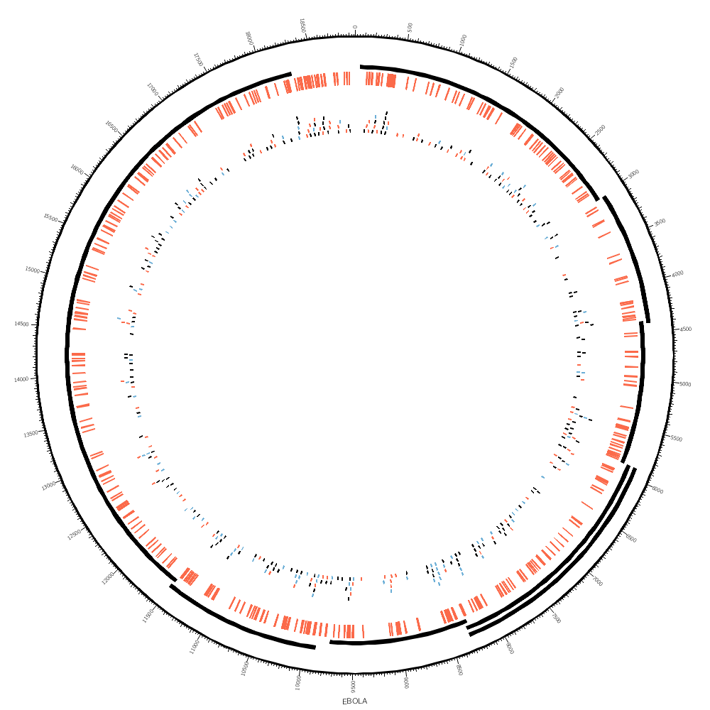
You'll see how you can use highlight and tile tracks to show regions and elements.
You'll see how rules can be used to color the SNPs, which are in the tile track. Since each SNP has a parameter snp (see the file above), you can test the value with a regular expression.
<rule>
condition = var(snp) =~ /^A/
color     = red
</rule>

<rule>
condition = var(snp) =~ /A$/
color     = blue
</rule>
The examples below show Circos installation filesystem paths from an older course. Your setup will be different but probably not that different.
Verify Perl and Circos installation
Both Perl and Circos have been installed on your workstation.
To verify that both are in your PATH
> which perl
/BGA2019/perl-5.24.1/bin/perl
> which circos
/BGA2019/circos-0.69-8/bin/circos
If which does not return anything, you'll need to load the module
> module use /BGA2019/modulefiles
> module load circos
Alternatively, you would have received the directory where Circos was installed and if it's not in your PATH, you'll need to add it. For example, if Circos is installed in /opt/circos-0.69-8 then to add the Circos binary to your PATH at the command line
>export PATH=$PATH:/opt/circos-0.69-8/bin
You should also add this to your .bashrc file.
Download and Install Course Materials
Course materials can be downloaded from
http://mkweb.bcgsc.ca/pasteur/italy.2019
To install the materials, untar the archive, assuming you've downloaded it into your home directory.
# switch to your home directory
> cd ~
> tar xvfz ~/circos.italy.2019.v1.10.tgz
There may be a more recent version of course materials than v1.10. Check the course website.
Course Materials File Organization
The structure of the course materials is as follows
circos/
  handouts/
  sessions/
    day.1/
        lecture.1/
            1/
            2/
            ...
        lecture.2/
            ...
Material is organized by day and lecture (1 day with 4 main lectures and 2 supplemental lectures). Each lecture has one or more independent sections. Here the term "lecture" covers both theoretical and practical lectures. All lectures except for the first one are practical sessions in which you'll be working at your workstation.
Using Course Files
During each lecture, you will be working entirely within the corresponding lecture directory.
For example, for Day 1 Lecture 2, you will be working from ~/circos/day.1/lecture.2
> cd circos/sessions/day.1/lecture.1
> ls
drwxr-xr-x 3 martink users 4096 Jun 15 21:02 1/
drwxr-xr-x 3 martink users 4096 Jun 15 21:02 2/
drwxr-xr-x 3 martink users 4096 Jun 15 21:02 3/
drwxr-xr-x 3 martink users 4096 Oct 15  2018 4/
drwxr-xr-x 3 martink users 4096 Jun 15 21:02 5/
drwxr-xr-x 3 martink users 4096 Jun 15 21:02 6/
drwxr-xr-x 3 martink users 4096 Jun 15 21:02 7/
-rw-r--r-- 1 martink users 1709 Jun 15 20:17 README
On the course website you'll see the content of each of the files listed. For example, right now you're reading day.1/lecture.1/README
You'll start each lecture by navigating to its first directory
> cd circos/sessions/day.1/lecture.2/1
-rw-r--r-- 1 martink users    912 Jun 15 12:35 README
-rw-r--r-- 1 martink users 228897 Jun 15 12:33 circos.png
drwxr-xr-x 2 martink users   4096 Jun 15 21:02 etc/
and follow along on the webpage for that lecture. The page will show the contents of relevant files in this directory, such as one or more READMEs, Circos configuration and any scripts.
Once you are done with first part of the lecture, move to the next part
> cd ../2
Circos Configuration Files
Many lecture parts will have a etc/ directory with one or more Circos configuration files that are used to generate images for the lecture.
The main file configuration file will be etc/circos.conf file and other configuration files will be imported from that directory or others that have files shared between lecture. This configuration file will import contents from other files, such as (a) configuration files shared by other lessons in this session, (b) configuration files shared by all sessions in this course and (c) predefined configuration files in the Circos distribution that define default parameters.
Files are imported using the <<include>> directive. The included file is defined relative to the configuration file in which the <<include>> directive is found.
Lecture Structure
The structure of each lecture is the same. Files for lectures are independent — what you did in the previous lesson does not affect the configuration file of the next lesson.
Follow along on the webpage for the lecture and load the files being discussed in your text editor. Typically this will be etc/circos.conf but sometimes we'll be working with etc/ideogram.conf or etc/ticks.conf. It will be easier if you can have each file open in a separate editor buffer, or window.
If there is a README you can follow it along in your browser or text editor. It's up to you.
When you read files in your text editor, you're see some formatting codes such as code, file and link. These are used by the webpage for formatting. It should be pretty obvious when you see it.
Once you have the file loaded in your editor, you'll typically see some comments in the file that explain what is happening and what to do.
Frequently, you'll be asked to modify the file either by entering new content or by uncommenting lines that are commented out (lines prefixed with #).
If we don't have time to cover all the parts for a lecture, I encourage you to finish them on your own.
Creating Circos images
For lecture parts that have etc/circos.conf, you'll be creating Circos images.
To do this
> cd ~/circos/sessions/day.1/lecture.2/1
> circos
debuggroup summary 0.31s welcome to circos v0.69-8 15 Jun 2019 on Perl 5.010000
...
debuggroup output 11.27s generating output
debuggroup output 11.33s created PNG image ./circos.png (229 kb)
> ls
-rw-r--r-- 1 martink users 912 Jun 15 12:35 README -rw-r--r-- 1 martink users 228897 Jun 15 21:32 circos.png drwxr-xr-x 2 martink users 4096 Jun 15 21:02 etc/
Now look at the circos.png file in a file viewer.
*** IMPORTANT ***
You need to run Circos from the directory lecture.2/1 and not from lecture.2/1/etc or any other directory.
This is because there are relative path file definitions in the configuration files that refer to lecture directories on other days and these are defined relative to lecture.2/1.
If you get a file-not-found error, such as the one below, it's likely that you're running Circos from the wrong directory.
Error parsing the configuration file. You used an <<include FILE>> directive,
but the FILE could not be found. This FILE is interpreted relative to the
configuration file in which the <<include>> directive is used. Circos lookd
for the file in these directories
Circos Errors
If Circos cannot find the configuration file, you'll see this error
  *** CIRCOS ERROR ***

  CONFIGURATION FILE ERROR

  Circos could not find the configuration file. To run Circos, you need to
  specify this file using the -conf flag. The configuration file contains all
  the parameters that define the image, including input files, image size,
  formatting, etc.

  If you do not use the -conf flag, Circos will attempt to look for a file
  circos.conf in several reasonable places such as . etc/ ../etc
Common Errors
Watch out for these common errors when editing the configuration file. Circos can identify some errors and produce a detailed message.
Missing Configuration File
If you run Circos without specifying the configuration file with -conf and Circos cannot locate the file (it tries in etc/, ../etc and a few other places) you'll see this error
  *** CIRCOS ERROR ***

  CONFIGURATION FILE ERROR

  Circos could not find the configuration file. To run Circos, you need to
  specify this file using the -conf flag. The configuration file contains all
  the parameters that define the image, including input files, image size,
  formatting, etc.

  If you do not use the -conf flag, Circos will attempt to look for a file
  circos.conf in several reasonable places such as . etc/ ../etc
You can see where Circos tried to look by using -debug_group io
> circos --debug_group io
Unbalanced Configuration Blocks
Make sure that you do not forget to close a block.
<rules>
 <rule>
 </rule>

 <rule>
</rules>
The missing </rule> for the second <rule> block will cause a parsing error. Don't forget closing </links>, </plots> and </rules> tags.
Redundant Parameter Definitions
In most cases you are not allowed to have multiple definitions of a parameter.
<plot>
..
color = black
..
color = red
..
</plot>
Circos will catch this and tell you what parameter is defined more than once.
CONFIGURATION FILE ERROR

  Configuration parameter [color] in parent block [plot] has been
  defined more than once in the block shown above, and has been interpreted as a
  list. This is not allowed. Did you forget to comment out an old value of the
  parameter?
Missing eval()
In a rule, if you want the parameter to be evaluated, don't forget eval().
<rule>
condition = 1
color = var(chr)
</rule>
This will set the color to var(chr) without evaluating it to the actual value of the chromosome. You want color = eval(var(chr))
When Circos does not recognize a color name it will default to black.
Debugging Circos
When things don't behave as you expect, you can use Circos' debugging facilities to narrow down the problem. Configuration Dump
Using the -cdump flag you can obtain the configuration file data structure. The output will reflect the hierarchical nature of the configuration file.
plots => {
           color => 'black',
           max => 1,
           min => 0,
           plot => [
                    {
                     file => '../data/both.cons.2e6.max.txt',
                     fill_color => 'spectral-5-div-3'
                    },
The output is large, and best combined with grep. For example, to search for all parameter that match cache,
> circos -cdump | grep cache
          color_cache_file => 'circos.colorlist',
          color_cache_static => 1,
Debug Groups
There is a large number of diagnostic reports that can be generated during image creation, named by the associated functionality. The reports can be accessed using -debug_group and combined as a list (e.g. io,conf,timer).
# reports about file location
>circos --debug_group io
# configuration file parsing and substitution
>circos --debug_group conf
# timings
>circos --debug_group timer
# all reports (long)
>circos --debug_group _all
For a list of report groups see
http://circos.ca/documentation/tutorials/configuration/debugging