All things Color — tools for understanding, choosing, designing and naming
contents
- 1 · Tools at a glance
- 2 · Color palettes for color blindness
- 3 · Color summarizer
- 4 · Maximally distinct colors
- 5 · Differences in color differences
- 6 · Lines of confusion in color blindness
- 7 · Brewer palette Adobe swatches
- 8 · List of named colors
- 9 · Color proportions in country flags
- 10 · Snap to colors and find colors
- 11 · Convert colors and white points between color spaces
palettes for color blindness — design advice for color blindess and 8-, 15- and 24- color palettes
colorsummarizer — cluster colors and create color summaries of an image
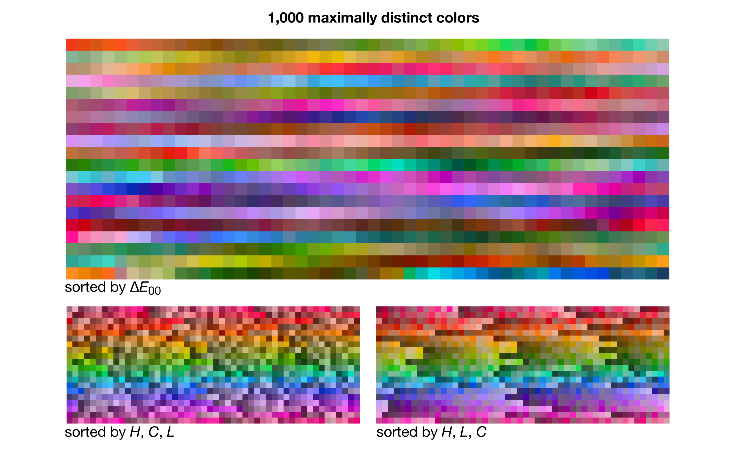
maximally distinct colors — lists of maximally distinct colors, from 5 to 3000!
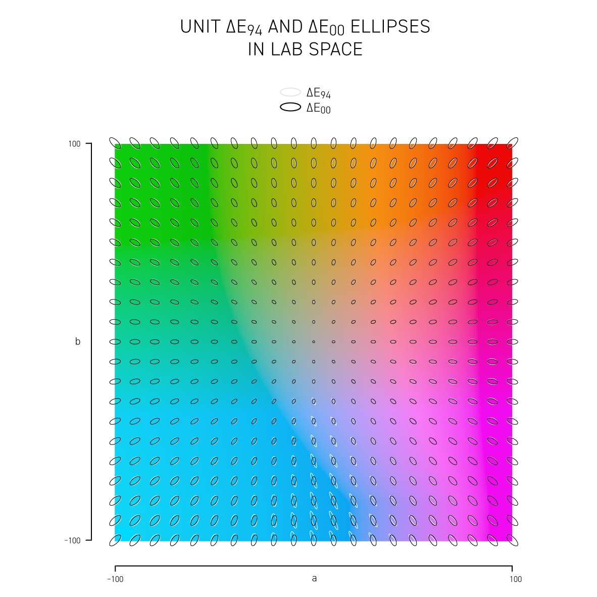
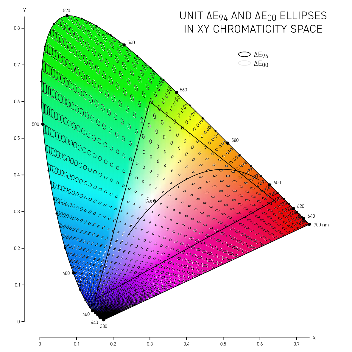
measurement of color differences — a comparison between color difference methods (`\Delta E_{94}` and `\Delta E_{00}`)
lines of confusion — math behind how equivalent colors in color blindness are calculated: lines of confusion and copunctal points
Adobe swatches for Brewer palettes — learn about Brewer palettes and import them into Illustrator and Photoshop
database of color names — names for over 8,300 colors
colors in country flags — proportions of colors in each country flag
colorsnap — replace colors in an image with a reference set of colors
colorconvert — convert colors between color spaces
These color resources are a side project and provided absolutely free to use with no restrictions. If you find them useful, your donation would be a way to say thanks.
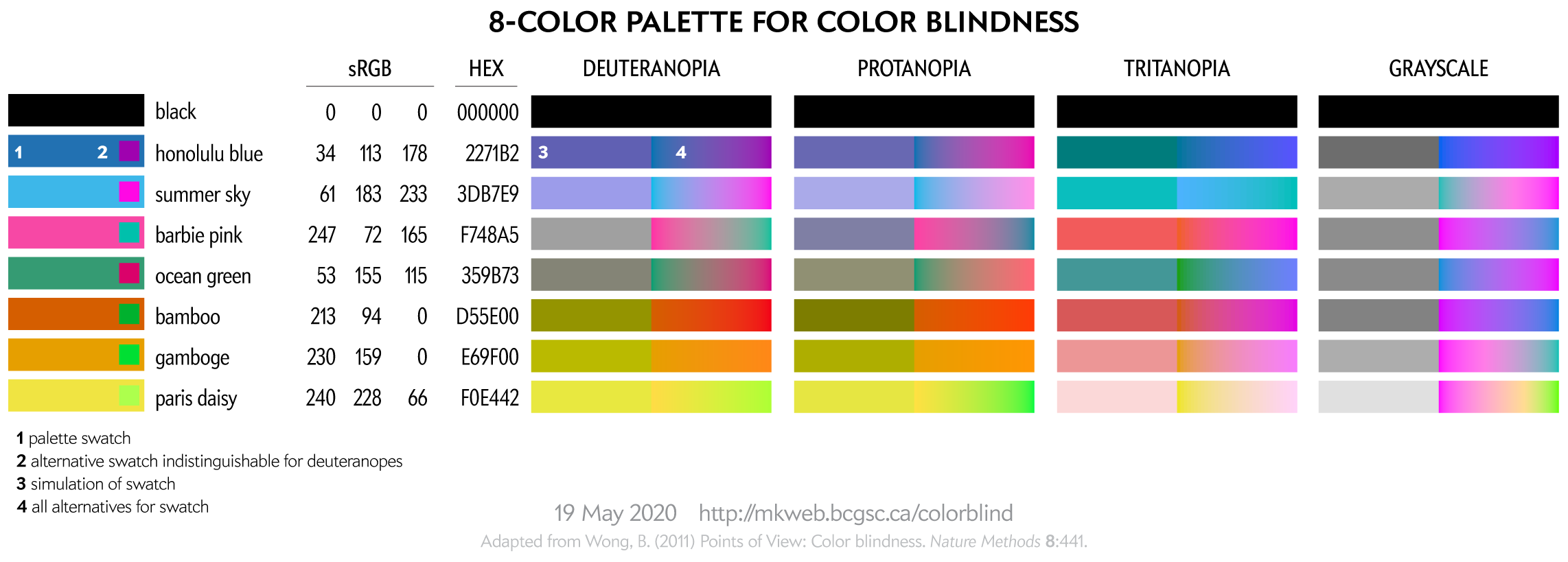
You should consider color blindness when you're designing and encoding information. Doing this will not only teach you more about color but expand the reach of your designs — both are a good thing.
I provide some background on color blindness and give options for choosing 8-, 12-, 15- and 24-color palettes that are color blind safe. I've also created a worksheet of color equivalencies that allows you to quickly create your own palette.
The palettes are suitable for categorical color encoding—the colors do not, as a whole, have a natural order and none is substantially more salient than another.
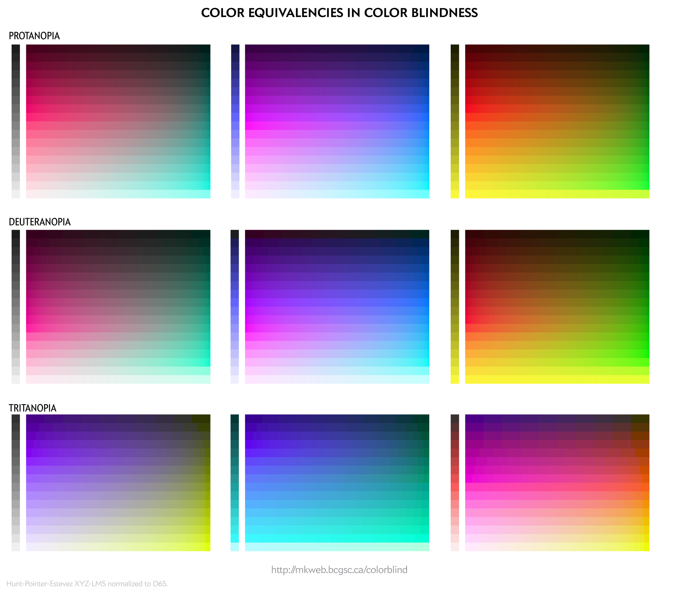
For a given color blindness type (e.g. deuteranopia) and channel (e.g. blue), the rows represent reasonably uniform steps in LCH luminance of the simulated color and a rich (high chroma) simulation at that luminance.
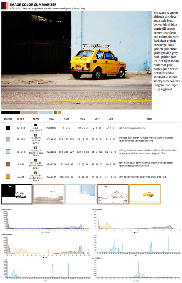
3 · Color summarizer
The color summarizer generates statistical color summaries of images. Whereas colorsnap (see above) calculates how close the colors in an image match a set of reference colors, colorsummarizer finds `k` such reference colors for which the difference compared to the image colors is minimum.
It reports average RGB, HSV, LAB and LCH color components as well as histograms and individual pixel values for these color spaces. Comes with useful web API for all your automation needs.
Yes! I support LCH, which is extremely useful in generating color ramps and, in general, talking about perceptual aspects of color that are intuitive.
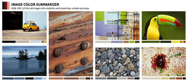
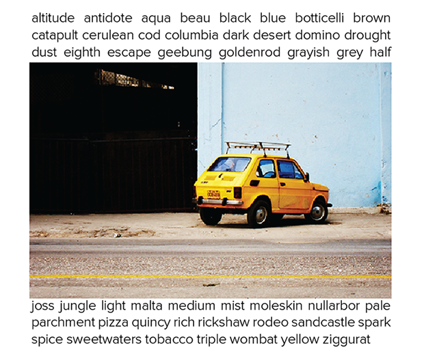
The color summarizer also identifies representative colors in the image by using k-means clustering to group colors into clusters. The centers of each cluster are also reported by name, using my large database of named colors.
Below is an example of a detailed color report of an image—an adorable Fiat 126p I found while it was screaming out its color against the fading background of Havana.
Color blindness is a thing. You should worry about it when you're designing and especially when you're encoding information. I provide some background on color blindness and give options for choosing 8-, 12-, 15- and 24-color palettes that are color-blind-safe. I've also created a worksheet of color equivalencies that allows you to quickly create your own palette.
The palettes are suitable for categorical color encoding—the colors do not, as a whole, have a natural order and none is substantially more salient than another.
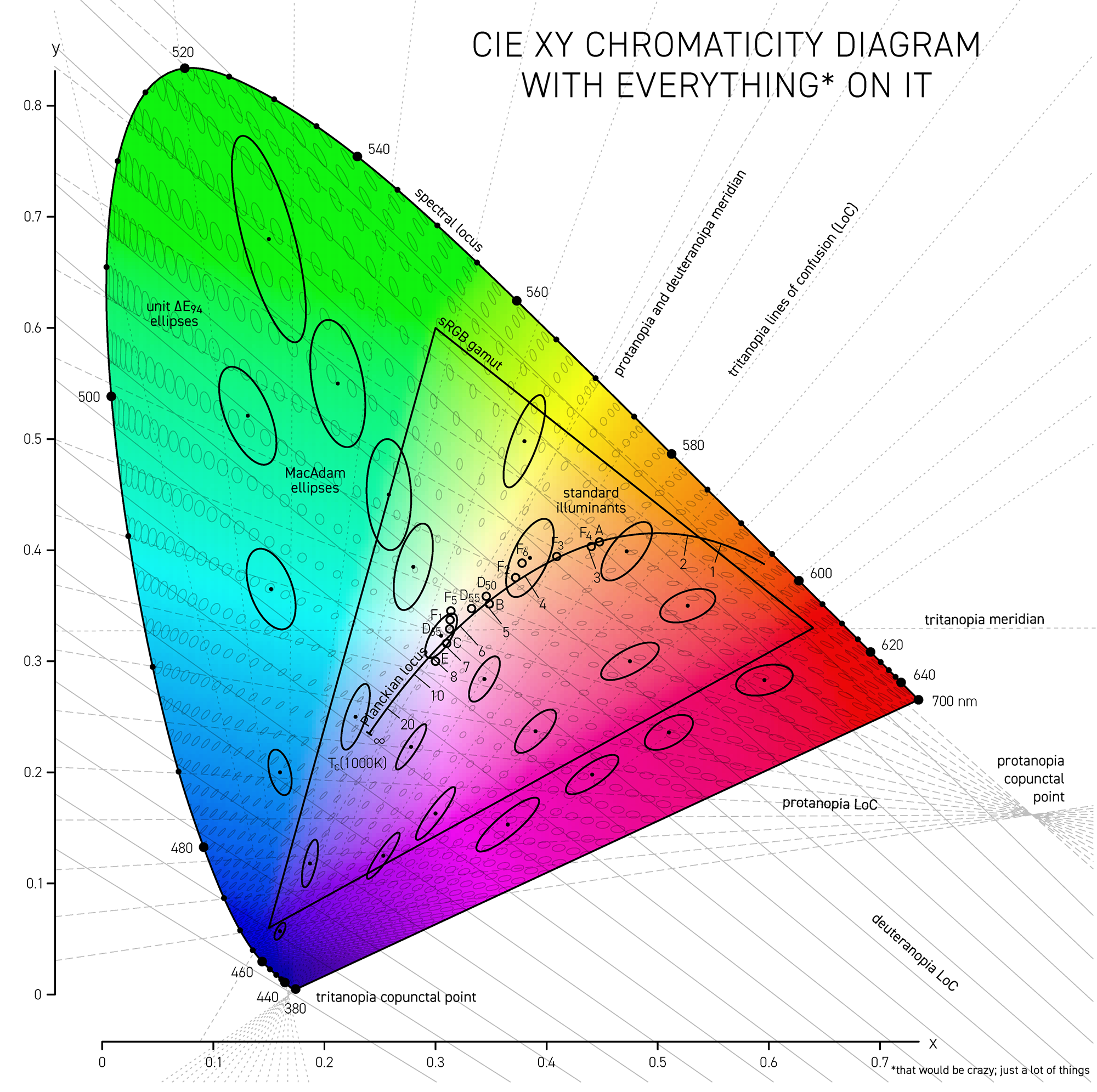
The difference between colors is called delta E (`\Delta E`) and is expressed by a number of different formulas — each slightly better at incorporating how we perceive color differences. I show how these vary in Lab space and CIE `xy` space.
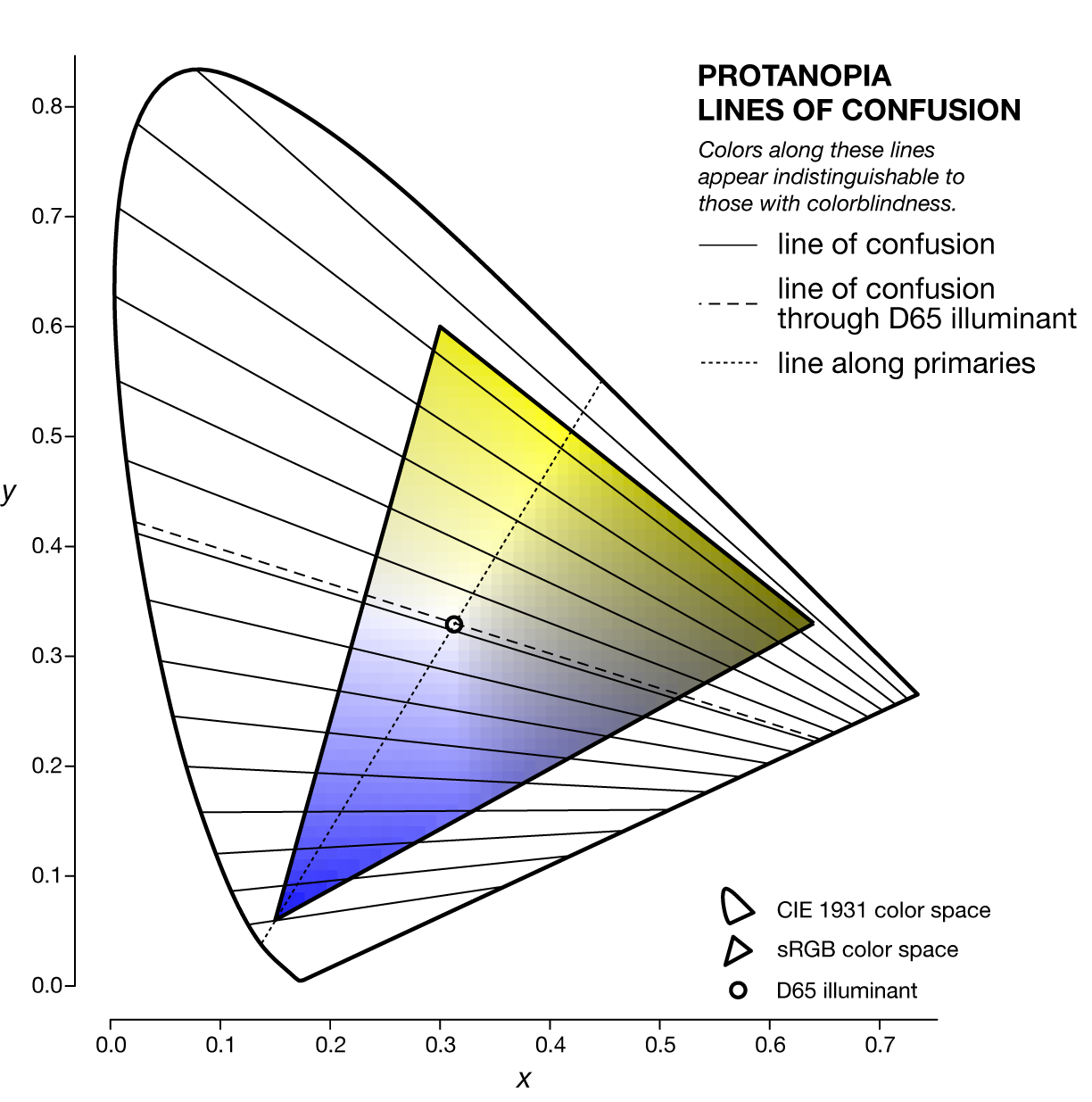
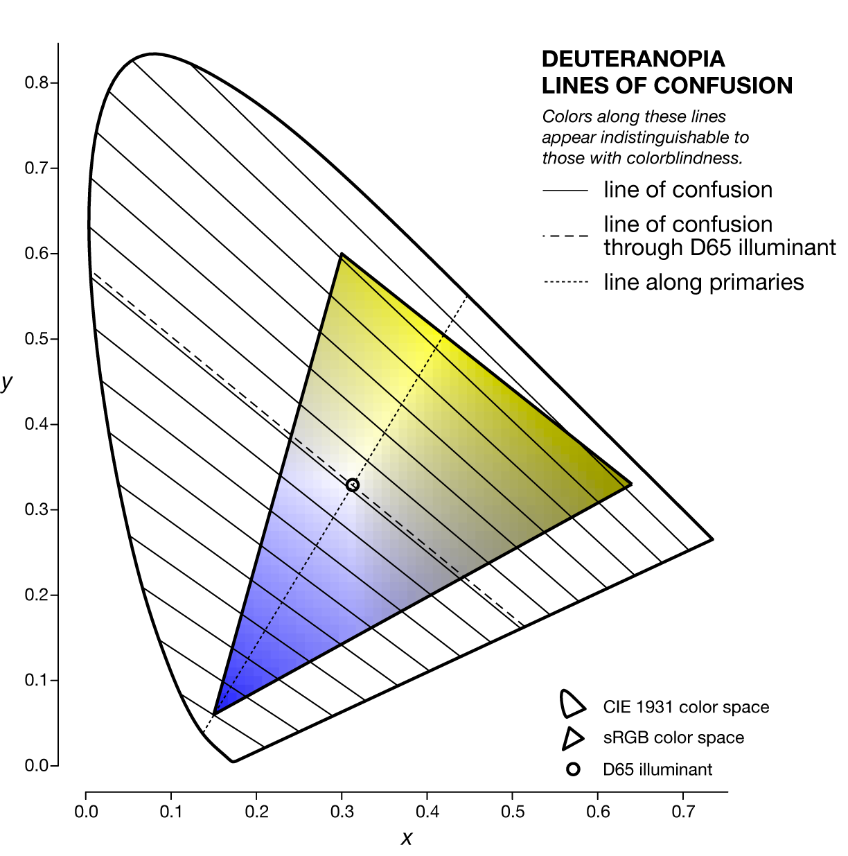
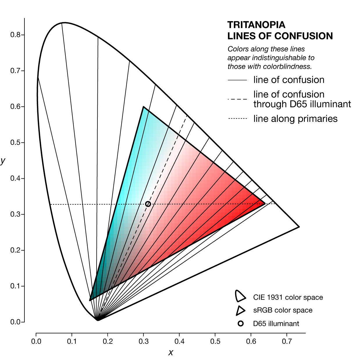
A line of confusion is the set of colors that appear identical to someone with color blindness. Each kind of color blindness has its own set of lines of confusion.
The specific line of confusion that passes through the white point divides the space into two hues. For example, for protanopes and deuteranopes these hues are blue and yellow but the line that divides the CIE space into the hues is slightly different. The figures below also show the line between the two color-blind primaries — the two colors that are not altered by the color blindness.
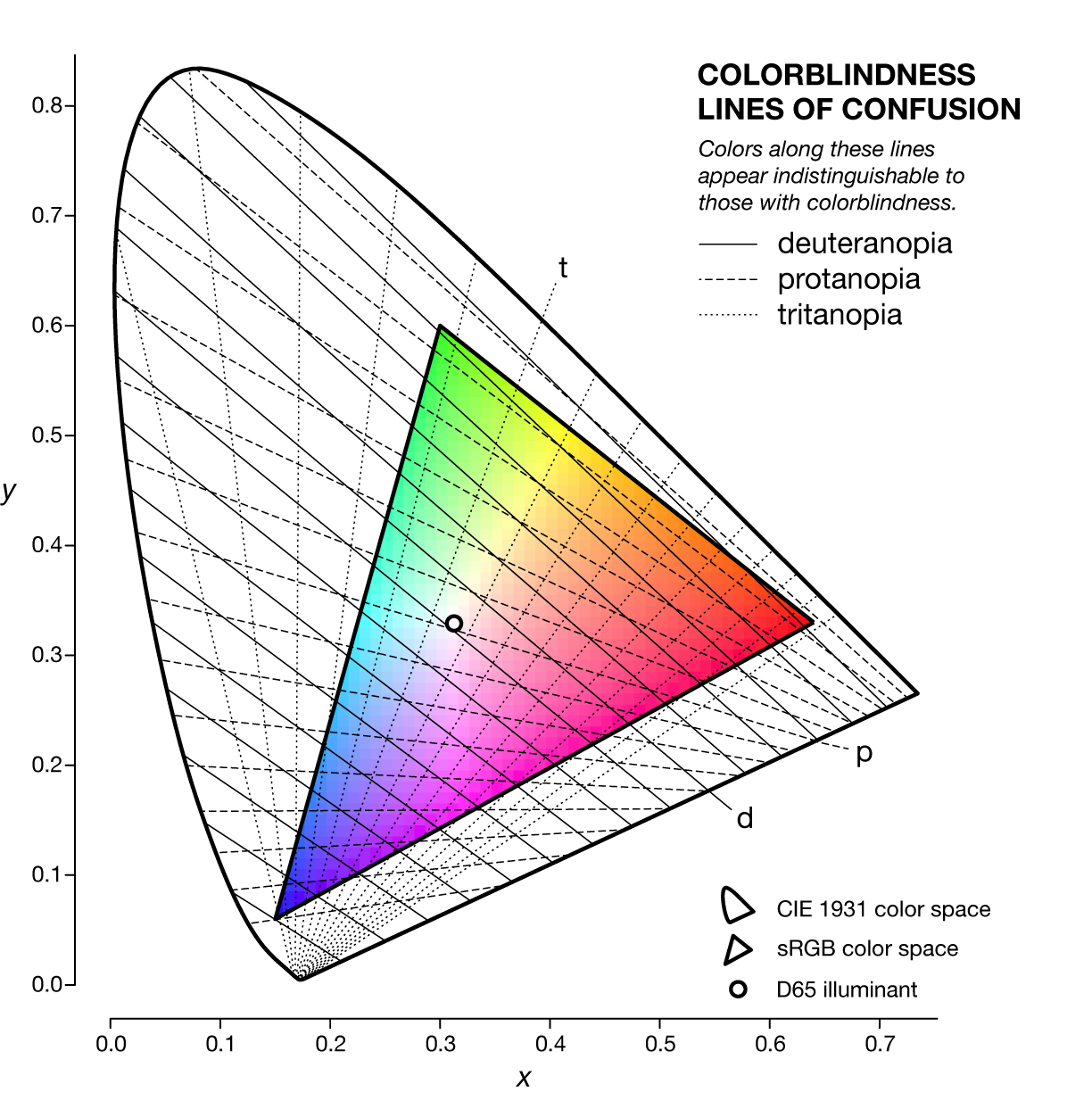
Each kind of color blindness has its own set of lines of confusion and all its lines of confusion go throught the copunctal point – the invisible color!
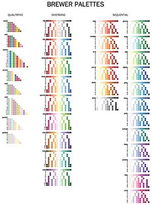
The Brewer color palettes are an excellent source for perceptually uniform color palettes. I provide Adobe Swatches for all colors in the Brewer Palettes.
I also provide a short talk to help you understand why these palettes are important.
Probably the world's largest list of named colors.
With more than 8,300 colors, even a mantis shrimp would be impressed. You can finally imagine a color you can't even imagine and name it!
The color name list is hooked into the color summarizer's clustering. You can get a list of words, derived from the color names, that describes an image.
A visual survey of the color proportions in flags of 256 countries.
Flags are depicted by concentric rings whose thickness is a function of the amount of that color in the flag.
I make the flag color catalog available, as well as similarity scores based on color proportions for each flag pair, so you can run your own analysis.
Download colorsnap
Linux/Win, v0.21 10 Feb 2021
The Gretag Macbeth color checker represented in sRGB D65 colors. Colors from RGB coordinates of the Macbeth colorchecker by D. Pascale (download colors).
If you want to find specific colors in an image or snap colors to a set of reference colors then my colorsnap application is for you (read documentation).
This application is useful if you want to figure out what fraction of an image is occupied by a specific color (or color range). The color clustering provided by the colorsummarizer is not useful in this case since the clustering does not key off specific colors. colorsnap will also report the average color of all snapped colors for each reference color and the `\Delta E` of the reference and average.
No shape or position analysis is performed whatsoever. Each pixel is snapped independently.
The application is written in Perl and runs natively on Linux. I've also created a compiled binary for Windows—no need to install Perl. It generates plain-text reports about color proportions, making it perfect for scripting and reports and analyzing the colors in a large number of images.
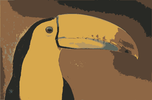
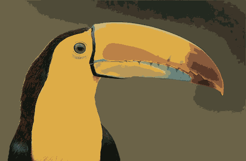
# man page
> bin/colorsnap -man

# snap tucan image and create snap image and histogram image
> bin/colorsnap -file tucan.jpg -delta_e_max 25 -snap -bar
As usual, for windows replace / in filepaths with \.
For example, the tucan image below was snapped to the 24 Gretag Macbeth colorchecker colors—each color in the original image was matched to the closest color in the colorchecker.
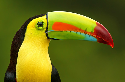
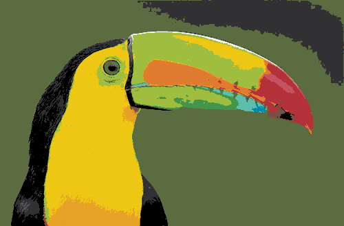
When snapping to reference colors you can impose a maximum color difference, as measured by `\Delta E`.
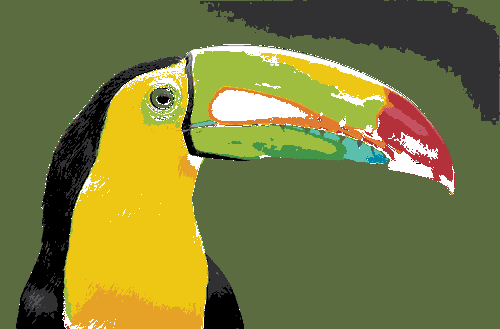
The application also generates a plain-text report of the color distribution—great for scripting and reports.
      black_2 rgbref  49  49  51 rgbavg  41  45  18 dE  19.7 n 17322  0.105  0.105  0.199 *****
         blue rgbref  35  63 147 rgbavg   -   -   - dE     - n     0  0.000  0.000  0.000
  blue_flower rgbref 130 128 176 rgbavg   -   -   - dE     - n     0  0.000  0.000  0.000
     blue_sky rgbref  91 122 156 rgbavg   -   -   - dE     - n     0  0.000  0.000  0.000
 bluish_green rgbref  92 190 172 rgbavg  79 164 145 dE   9.6 n   716  0.004  0.004  0.008
         cyan rgbref   0 136 170 rgbavg  50 139 143 dE  17.8 n   139  0.001  0.001  0.002
    dark_skin rgbref 116  81  67 rgbavg  85  36  10 dE  22.5 n   655  0.004  0.004  0.008
      foliage rgbref  90 108  64 rgbavg  68  83  15 dE  16.5 n 86944  0.529  0.529  1.000 ***********************
        green rgbref  67 149  74 rgbavg  82 136  34 dE  15.9 n  1390  0.008  0.008  0.016
   light_skin rgbref 199 147 129 rgbavg 219 150 131 dE   7.8 n    61  0.000  0.000  0.001
      magenta rgbref 193  84 151 rgbavg   -   -   - dE     - n     0  0.000  0.000  0.000
 moderate_red rgbref 198  82  97 rgbavg 176  87  80 dE  13.6 n   490  0.003  0.003  0.006
  neutral_3.5 rgbref  82  84  86 rgbavg  73  81  77 dE   5.0 n   268  0.002  0.002  0.003
    neutral_5 rgbref 121 121 122 rgbavg 111 120 113 dE   6.1 n    91  0.001  0.001  0.001
  neutral_6.5 rgbref 161 163 163 rgbavg 149 164 142 dE  13.3 n    99  0.001  0.001  0.001
    neutral_8 rgbref 200 202 202 rgbavg 200 205 171 dE  18.0 n    51  0.000  0.000  0.001
       orange rgbref 224 124  47 rgbavg 218  79   6 dE  21.6 n  3853  0.023  0.023  0.044 *
orange_yellow rgbref 230 162  39 rgbavg 186 145   4 dE  14.3 n  4466  0.027  0.027  0.051 *
   pure_black rgbref   0   0   0 rgbavg  24  17   7 dE   7.9 n  7856  0.048  0.048  0.090 **
   pure_white rgbref 255 255 255 rgbavg   -   -   - dE     - n     0  0.000  0.000  0.000
       purple rgbref  94  58 106 rgbavg  32  42  80 dE  20.8 n     2  0.000  0.000  0.000
purplish_blue rgbref  68  91 170 rgbavg   -   -   - dE     - n     0  0.000  0.000  0.000
          red rgbref 180  49  57 rgbavg 139  27  18 dE  15.6 n  3512  0.021  0.021  0.040 *
    white_9.5 rgbref 245 245 243 rgbavg 251 251 202 dE  23.8 n   371  0.002  0.002  0.004
       yellow rgbref 238 198  20 rgbavg 239 217  43 dE  10.1 n 24507  0.149  0.149  0.282 ********
 yellow_green rgbref 159 189  63 rgbavg 169 194  36 dE  11.3 n 11707  0.071  0.071  0.135 ****
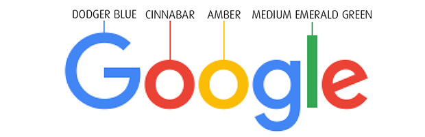
You can uses this application for quick and easy image color analysis. For example, by using the Google maps traffic density colors, you can snap the colors in a Google map to these colors (disregarding all others) to get a sense of the fraction of streets that are busy.
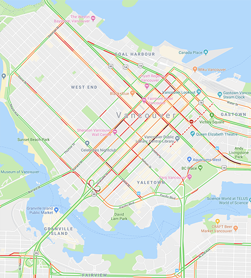
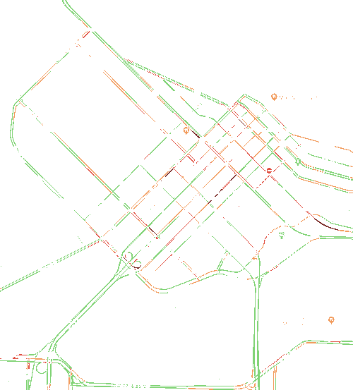
   dred rgb 119  39  35 n  203  0.018  0.001  0.028
  green rgb 128 211 117 n 7210  0.656  0.026  1.000 ******************************
   lred rgb 224  76  62 n  992  0.090  0.004  0.138 ****
 orange rgb 242 155  92 n 2581  0.235  0.009  0.358 **********
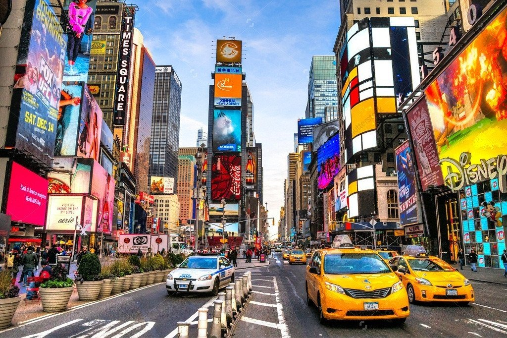
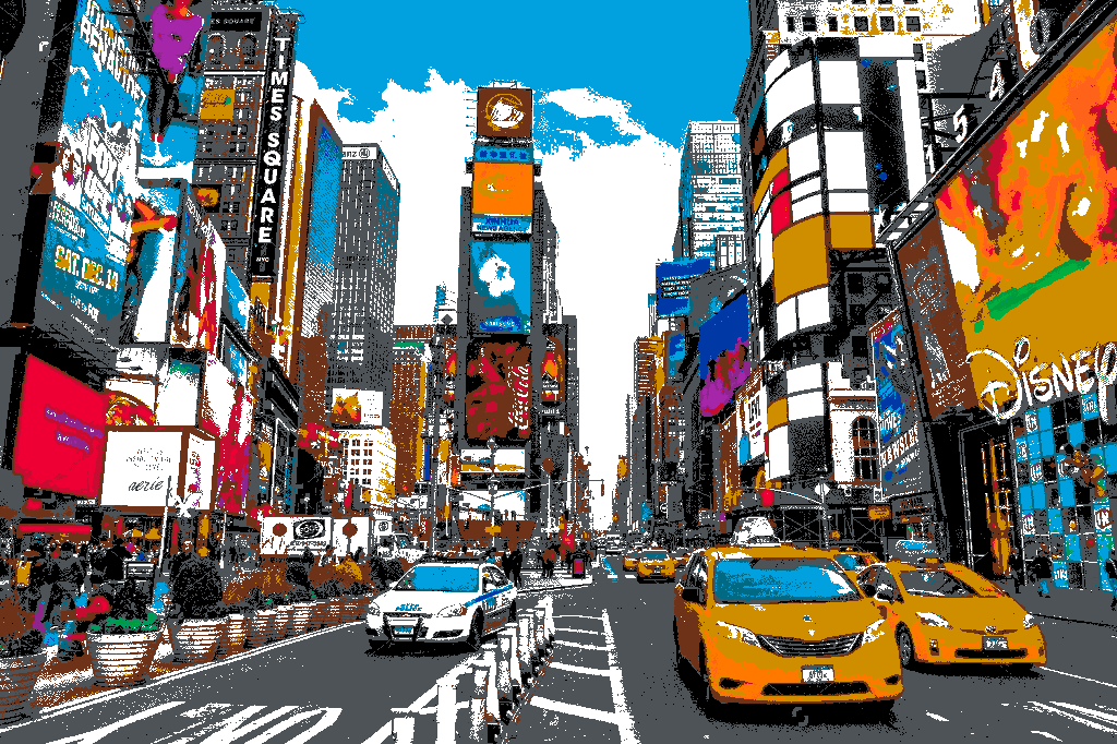
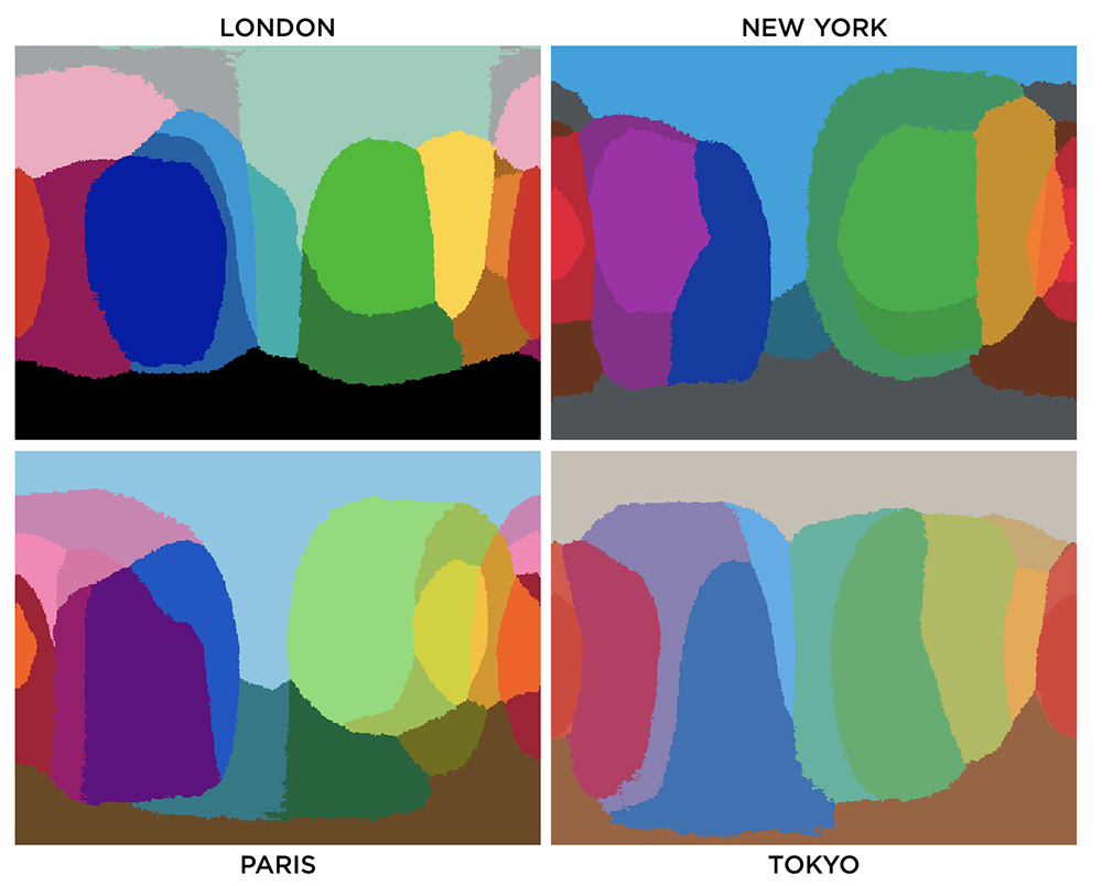
You can use colorsnap to convert artwork to a different palette. For example, below are the colors of the subway lines in New York City, Paris and London.
Colors used by the New York MTA subway lines.
Colors used by the Paris metro lines.
Colors used by the London underground lines.
Colors used by the Tokyo subway lines.
Below is an image of Times Square in New York City snapped to the New York City subway line colors
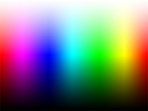
The Granger rainbow gives a concrete example of how snapping works.
This rainbow is a color calibration image and contains all the RGB colors—here resized as a small image so strictly not all colors are present.
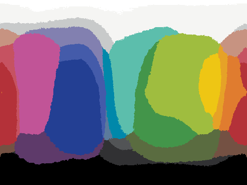
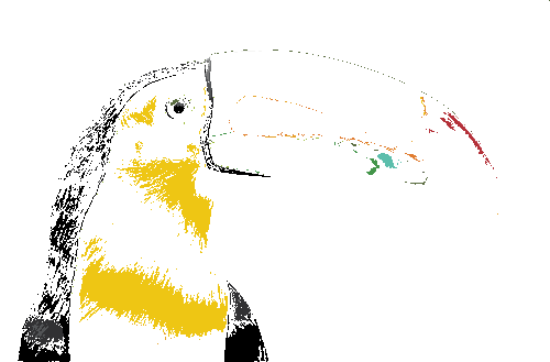
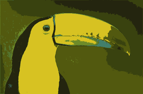
One way of deriving the reference colors is to use colorsummarizer to cluster colors in oine image and then using the average cluster color as the input for colorsnap for a different image. Let's try this with the tucan image with Munch's Scream as the reference.
`k=8` means clusters for Munch's Scream (download colors).
`k=32` means clusters for Munch's Scream (download colors).
Above are the swatches for each of the `k=8` and `k=32` clusters of The Scream as analyzed by my colorsummarizer image clustering tool. Below are the colorsnap results for the tucan image using `k=8` cluster colors.
 barley_corn rgbref 185 153  98 rgbavg 110 139  41 dE  34.5 n  3047  0.019  0.019  0.057 *
 brown_derby rgbref  88  68  52 rgbavg  57  66  15 dE  24.1 n 34665  0.211  0.211  0.643 ************
  brown_grey rgbref 143 131 105 rgbavg  84 116  46 dE  32.2 n  2403  0.015  0.015  0.045
 brown_sugar rgbref 142 103  69 rgbavg  82  89  15 dE  29.7 n 53898  0.328  0.328  1.000 ********************
       cello rgbref  57  80  97 rgbavg  60  76  83 dE   6.7 n    49  0.000  0.000  0.001
jungle_green rgbref  40  41  37 rgbavg  36  37  15 dE  12.2 n 25368  0.154  0.154  0.471 *********
   limed_ash rgbref  94 102  92 rgbavg  66 127 107 dE  20.8 n  1387  0.008  0.008  0.026
     rob_roy rgbref 215 168  77 rgbavg 215 194  34 dE  27.4 n 43683  0.266  0.266  0.810 ****************
Download colorconvert
Linux/Win, v0.10 10 Feb 2021
The colorconvert (read documentation) converts colors between color spaces, white points and RGB working spaces.
colorconvert is very useful for analyzing and transforming color coordinates. The output can be easily parsed by downstream scripts or imported into a spreadsheet. You can read colors from a file.
For example, you can use colorconvert to get the RGB and XYZ color coordinates of all white points at each color temperature in the range 4,000–25,000 K.
bin/colorconvert -from 4000K -to RGB255,RGBhex,xyz -oneline
bin/colorconvert -from 4050K -to RGB255,RGBhex,xyz -oneline
...
bin/colorconvert -from 25000K -to RGB255,RGBhex,xyz -oneline
See the bin/whitepoints.sh script.
The tool has support for the following color spaces: RGB XYZ xyY Lab LCHab Luv LCHuv HSL HSV CMY CMYK YCbCr YPbPr YUV YIQ LMS, RGB working spaces: 601, 709, Adobe, Adobe RGB (1998), Apple, Apple RGB, BestRGB, Beta RGB, BruceRGB, CIE, CIE ITU, CIE Rec 601, CIE Rec 709, ColorMatch, DonRGB4, ECI, Ekta Space PS5, NTSC, PAL, PAL/SECAM, ProPhoto, SMPTE, SMPTE-C, WideGamut, sRGB white points: A B C D50 D55 D65 D75 D93 E F11 F2 F7 4000K-25000K.
# convert an RGB color to all color spaces
> bin/colorconvert -from 41,171,226
RGB255       41      171      226
RGBhex   29ABE2
   RGB    0.161    0.671    0.886
   XYZ    0.292    0.351    0.772
   xyY    0.206    0.248    0.351
   Lab   65.815  -15.265  -37.260
 LCHab   65.815   40.266 -112.279
   Luv   65.815  -42.283  -57.421
 LCHuv   65.815   71.309 -126.367
   HSL  197.838    0.761    0.524
   HSV  197.838    0.819    0.886
   CMY    0.839    0.329    0.114
  CMYK    0.725    0.216        0    0.114
 YCbCr  148.295  156.939   98.634
 YPbPr    0.604    0.129   -0.131
   YUV    0.604    0.113   -0.161
   YIQ    0.604   -0.197    0.007
   LMS    0.230    0.410    0.782

# convert a Lab color to RGB255 and RGBhex using Adobe RGB working space
# with single-line CSV output
> bin/colorconvert -from lab,50,-25,50 -to RGB255,RGBhex -oneline -csv -to_rgb Adobe
RGB255 109,128,39 RGBhex 6D8027

# get coordinates of white point for 4000K in RGB255 and RGBhex
# with single-line CSV output
> bin/colorconvert -from 4000K -to RGB255,RGBhex -oneline -csv
RGB255 255,248,187 RGBhex FFF8BB

# convert colors from file
> bin/colorconvert -from spectral.15.txt -to RGBhex -oneline
spectral-15-div-1 RGBhex 9E0142
spectral-15-div-2 RGBhex D53E4F
spectral-15-div-3 RGBhex D7191C
...
Nasa to send our human genome discs to the Moon
We'd like to say a ‘cosmic hello’: mathematics, culture, palaeontology, art and science, and ... human genomes.


Comparing classifier performance with baselines
All animals are equal, but some animals are more equal than others. —George Orwell
This month, we will illustrate the importance of establishing a baseline performance level.
Baselines are typically generated independently for each dataset using very simple models. Their role is to set the minimum level of acceptable performance and help with comparing relative improvements in performance of other models.

Unfortunately, baselines are often overlooked and, in the presence of a class imbalance5, must be established with care.
Megahed, F.M, Chen, Y-J., Jones-Farmer, A., Rigdon, S.E., Krzywinski, M. & Altman, N. (2024) Points of significance: Comparing classifier performance with baselines. Nat. Methods 20.
Happy 2024 π Day—
sunflowers ho!
Celebrate π Day (March 14th) and dig into the digit garden. Let's grow something.

How Analyzing Cosmic Nothing Might Explain Everything
Huge empty areas of the universe called voids could help solve the greatest mysteries in the cosmos.
My graphic accompanying How Analyzing Cosmic Nothing Might Explain Everything in the January 2024 issue of Scientific American depicts the entire Universe in a two-page spread — full of nothing.

The graphic uses the latest data from SDSS 12 and is an update to my Superclusters and Voids poster.
Michael Lemonick (editor) explains on the graphic:
“Regions of relatively empty space called cosmic voids are everywhere in the universe, and scientists believe studying their size, shape and spread across the cosmos could help them understand dark matter, dark energy and other big mysteries.
To use voids in this way, astronomers must map these regions in detail—a project that is just beginning.
Shown here are voids discovered by the Sloan Digital Sky Survey (SDSS), along with a selection of 16 previously named voids. Scientists expect voids to be evenly distributed throughout space—the lack of voids in some regions on the globe simply reflects SDSS’s sky coverage.”
voids
Sofia Contarini, Alice Pisani, Nico Hamaus, Federico Marulli Lauro Moscardini & Marco Baldi (2023) Cosmological Constraints from the BOSS DR12 Void Size Function Astrophysical Journal 953:46.
Nico Hamaus, Alice Pisani, Jin-Ah Choi, Guilhem Lavaux, Benjamin D. Wandelt & Jochen Weller (2020) Journal of Cosmology and Astroparticle Physics 2020:023.
Sloan Digital Sky Survey Data Release 12
Alan MacRobert (Sky & Telescope), Paulina Rowicka/Martin Krzywinski (revisions & Microscopium)
Hoffleit & Warren Jr. (1991) The Bright Star Catalog, 5th Revised Edition (Preliminary Version).
H0 = 67.4 km/(Mpc·s), Ωm = 0.315, Ωv = 0.685. Planck collaboration Planck 2018 results. VI. Cosmological parameters (2018).
constellation figures
stars
cosmology
Error in predictor variables
It is the mark of an educated mind to rest satisfied with the degree of precision that the nature of the subject admits and not to seek exactness where only an approximation is possible. —Aristotle
In regression, the predictors are (typically) assumed to have known values that are measured without error.
Practically, however, predictors are often measured with error. This has a profound (but predictable) effect on the estimates of relationships among variables – the so-called “error in variables” problem.

Error in measuring the predictors is often ignored. In this column, we discuss when ignoring this error is harmless and when it can lead to large bias that can leads us to miss important effects.
Altman, N. & Krzywinski, M. (2024) Points of significance: Error in predictor variables. Nat. Methods 20.
Background reading
Altman, N. & Krzywinski, M. (2015) Points of significance: Simple linear regression. Nat. Methods 12:999–1000.
Lever, J., Krzywinski, M. & Altman, N. (2016) Points of significance: Logistic regression. Nat. Methods 13:541–542 (2016).
Das, K., Krzywinski, M. & Altman, N. (2019) Points of significance: Quantile regression. Nat. Methods 16:451–452.