Learning Circos
Bioinformatics and Genome Analysis
Fondazione Edmund Mach, San Michele all'Adige, Italy, 20 June 2019
v2.00 16 June 2019 Download PDF slides
v2.00 16 June 2019
A 1-day practical course in genomic data visualization with Circos. This material is part of the Bioinformatics and Genome Analysis course held at the Fondazione Edmund Mach in San Michele all'Adige, Italy. Materials also available here: course materials and PDF slides.
Quick links
MyPads | BCGA 2019 | 4-day Circos course | Circos documentation best practices getting started | Brewer palettes | Color resources | Nature Methods Points of View Points of Significance
Genomic Data Visualization with Circos
Thursday 20 June 2019 — Day 1
09h00 – 10h30 | Lecture 1 — Introduction to Circos
11h00 – 12h30 | Lecture (practical) 2 — Visualizing gene distribution and size in Yeast—the histogram data track
14h00 – 15h30 | Lecture (practical) 3 — Conservation in Yeast—the link data track
16h00 – 18h00 | Lecture (practical) 4 — Drawing the human genome
18h15 – 19h30 | Lecture (practical) 5 — Afterhours—Perl refresher
18h15 – 19h30 | Lecture (practical) 6 — Afterhours—Visualizing an Ebola strain
Concepts covered today
Circos configuration, common Circos errors, Circos debugging, ideograms, selecting ideograms with regular expressions, input data format, creating Circos data files, data tracks (histograms, heat map, tiles, links), color definitions and using transparency, Brewer palettes, dynamic data formatting rules, downloading files from UCSC genome browser, essential command-line tools and basic scripting,
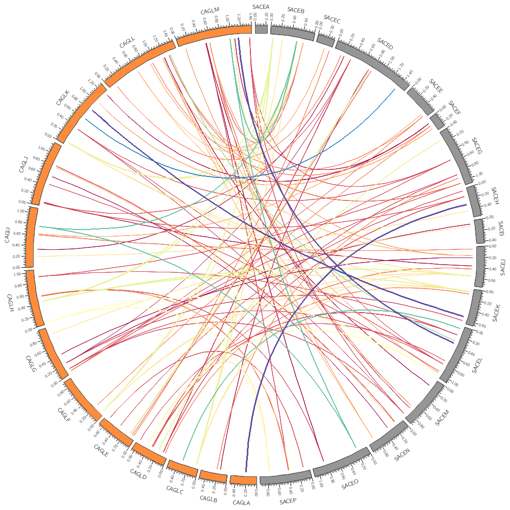
Conservation in Yeast—the link data track
Let's now look at how to draw links. These are useful for showing alignments and any other kind of similarity (or more generally, relationship) between two positions.
Let's draw chromosomes from a couple of the genomes, SACE and CAGL.
Here the regular expression is using the alternation pipe, meaning that chromosome names can match either sace or cagl.
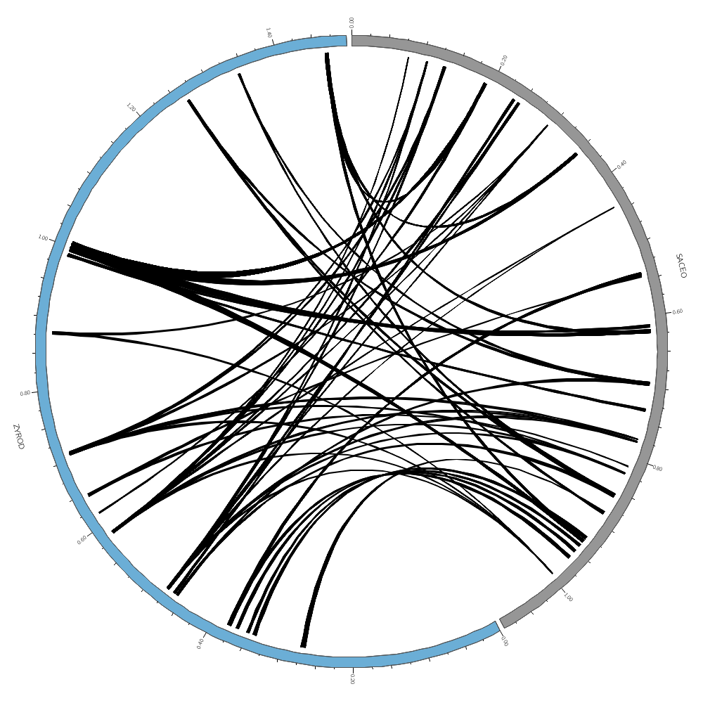
Once you've worked through this example, go back here and limit the display to only zyro-d and sace-o. Turn off the rule that hides 95% of the data.
Which chromosome combination in ../../data/links.conservation.10000.txt appears most frequently? Hint: parse the file with cut, sort and uniq to answer this question.
chromosomes_display_default = no
chromosomes = /sace|cagl/
Like plots, links are defined in blocks, except they go in <links> blocks. Individual link tracks have their own <link> block. Each line of a link data file defines two intervals: the start and end of the link.
# CHR1 START1 END1 CHR2 START2 END2
zyro-d 540803 555583 sace-l 349006 363738
zyro-d 540803 555583 sace-l 349006 363738
zyro-d 540803 555583 cagl-m 1143091 1157733
zyro-d 540803 555583 cagl-m 1143091 1157733
...
<links>
<link>
file          = ../../data/links.conservation.10000.txt
As you saw with histograms and heat maps, different plots expect different parameters. For links, you need to define the position of the ends of the links with the radius parameter. This is best done relative to the ideogram of the circle.
So here our links will go as far as 98% of the radius of the ideogram circle.
radius = 0.98r
This controls how curved the links are. Specifically, this is the radius of the control point. Try setting this to a larger value like 0.25r or 0.5r.
bezier_radius = 0r
Since there are 10,000 links in the file, the image might take a while to draw. The record_limit parameter is useful for limiting the number of entries read from the file for debugging. You activate this if the image is taking a long time to draw. record_limit = 1000
color         = black
thickness     = 1
If you have a large data set and only want to show a random subset of the data, you can define a rule that turns the display of the data point off show = no for a fraction of the data. Here, the rand() function returns a uniformly distributed number in the interval [0,1). This number will be < 0.95 exactly 95% of the time. The condition is evaluated for each data point and will be true, on average, for 95% of the data points, which will not be shown.
The difference between this and record_limit is that here we're sampling a random subset of the data, whereas record_limit draws the data subset from the start of the file.
Activate the rules by commenting out use = no or setting use = yes and play with the cutoff fraction.
<rules>
use       = no
<rule>
condition = rand() < 0.95
show      = no
</rule>
</rules>
Uncomment these when you're drawing zyro-d vs sace-o. The links will be drawn as ribbons (with no twist in the middle). ribbon = yes flat = yes
</link>
</links>
Input data format
Let's look in more detail at the data input files. Their format is relatively straightforward.
First, there are only two kinds of input data files. The first kind is used by (x,y)-style tracks such as line plots, histograms, heatmaps, tiles and so on. These tracks assign a value to a region on a chromosome. The format for this is
CHR START END VALUE {options}
For example, our histogram of average gene sizes in 10 kb bins looks like this
# day.1/data/genes.avgsize.10kb.txt
cagl-a 10000 19999 840
cagl-a 20000 29999 1661.4
cagl-a 30000 39999 1652.4
cagl-a 40000 49999 1828
cagl-a 50000 59999 2535
cagl-a 60000 69999 1856.4
...
If you use this file for a histogram track, the bins will be horizontal bars whose width is defined by the start and end coordinates. If you use this file for a scatter plot, then the point will be placed at the midpoint of the interval. Generally, the fourth column is the value that's used by the track and mapped onto a property, such as bar height.
It's important to stress here that the same data file can be used for various track types or reused for multiple tracks.
We'll worry about the {options} column later. This column can store additional property of the data point, such as a formatting property (color, thickness and so on, which may easily be adjusted by rules) or additional values that might be used for filtering in the track.
The second type of input file stores pairwise relationships between positions. Link files are of this form and have the format
CHR1 START1 END1 CHR2 START2 END2 {options}
For example, the conserved regions between SACE and CAGL used for the link track in this lecture are stored like this
# day.1/data/links.conservation.txt
cagl-a 19487 21757 sace-g 450197 452104
cagl-a 22260 24440 sace-g 452404 454560
cagl-a 25241 27622 sace-b 207194 209224
cagl-a 25241 27622 sace-g 454785 457067
cagl-a 27915 28586 sace-g 457163 457870
...
Creating a Circos figure generally begins with filtering your data set for the kinds of things you want to display and then generating the data files from them. We'll do this in the last lecture today.
In the previous section, we draw data from day.1/data/links.conservation.10000.txt, which contained the largest 10,000 conservation regions.
What is the distribution of sizes of all the links? To answer this, use the histogram script in this directory.
> ./histogram -help
Usage:
      cat numbers.txt | ./histogram [-help] [-man]

      cat numbers.txt | ./histogram -min 0 -max 100
      cat numbers.txt | ./histogram -min 0 -max 100 -binsize 10
      cat numbers.txt | ./histogram -min 0 -max 100 -nbins 20
Let's create a histogram of the sizes of the start of all the conservation links. We're going to assume that the end of the links is similarly sized.
We can use awk to parse out the start and end positions and report the size.
> cat ../../data/links.conservation.txt | awk '{print $3-$2+1}' | ./histogram
             159.0000>     0  0.000
  159.0000   890.1000  13291  0.126  0.126 ********
  890.1000  1621.2000  37458  0.356  0.482 *************************
 1621.2000  2352.3000  26369  0.251  0.733 *****************
 2352.3000  3083.4000  13276  0.126  0.859 ********
 3083.4000  3814.5000   7541  0.072  0.930 *****
 3814.5000  4545.6000   3550  0.034  0.964 **
 4545.6000  5276.7000   2656  0.025  0.989 *
 5276.7000  6007.8000    577  0.005  0.995
 6007.8000  6738.9000    226  0.002  0.997
 ...
       n       105263
 average   1925.13292
      sd   1135.06149
     min    159.00000
     max  14781.00000
     sum 202645267.00000
So, we have 105,263 links in the entire conservation set. Their start interval average is about 1.9 kb.
To get a better look, let's create a histogram in the range [0,5000] with a bin size of 250
> cat ../../data/links.conservation.txt | awk '{print $3-$2+1}' | ./histogram -min 0 -max 5000 -bin 250
               0.0000>     0  0.000
    0.0000   250.0000    197  0.002  0.002
  250.0000   500.0000   3119  0.030  0.032 *****
  500.0000   750.0000   6557  0.063  0.095 ************
  750.0000  1000.0000   9606  0.093  0.188 ******************
 1000.0000  1250.0000  12679  0.122  0.310 ************************
 1250.0000  1500.0000  11844  0.114  0.425 **********************
 1500.0000  1750.0000  13019  0.126  0.550 *************************
 1750.0000  2000.0000   9172  0.089  0.639 *****************
 2000.0000  2250.0000   6685  0.065  0.703 ************
 2250.0000  2500.0000   7831  0.076  0.779 ***************
 2500.0000  2750.0000   5411  0.052  0.831 **********
 2750.0000  3000.0000   3809  0.037  0.868 *******
 3000.0000  3250.0000   3026  0.029  0.897 *****
 3250.0000  3500.0000   2743  0.026  0.924 *****
 3500.0000  3750.0000   1877  0.018  0.942 ***
 3750.0000  4000.0000   1131  0.011  0.953 **
 4000.0000  4250.0000    893  0.009  0.961 *
 4250.0000  4500.0000   1587  0.015  0.977 ***
 4500.0000  4750.0000   1427  0.014  0.990 **
 4750.0000  5000.0000   1004  0.010  1.000 *
            5000.0000<  1646  0.016
You can see that roughly 90% (89.7%) of the links have a start interval size of < 3.25 kb.
Create a histogram of link size distributions in links.duplication.txt. What's the smallest link? What's the largest? How does this compare to the conserved link distribution?
The business part of the histogram script is shown below. Feel free to review it if you feel you have time.
# read the values from STDIN and use the -col COLUMN, by default 0
my @values;
while(my $line = <>) {
  chomp $line;
  next if $line =~ /^\#/;
  my @tok = split(" ",$line);
  if(defined $CONF{col} && ! defined $tok[ $CONF{col} ]) {
    die "The line [$line] has no number in column [$CONF{col}]";
  }
  push @values, $tok[ $CONF{col}];
}

# get min and max of values
my ($min,$max) = minmax(@values);

# change min/max range if redefined via -min and/or -max
$min = $CONF{min} if defined $CONF{min};# && $CONF{min} > $min;
$max = $CONF{max} if defined $CONF{max};# && $CONF{max} < $max;

# *very* quick and dirty percentile if -pmin or -pmax used
if($CONF{pmin} || $CONF{pmax}) {
  my @sorted = sort {$a <=> $b} @values;
  $min = $sorted[ $CONF{pmin}/100 * (@sorted-1) ] if $CONF{pmin};
  $max = $sorted[ $CONF{pmax}/100 * (@sorted-1) ] if $CONF{pmax};
}

# determine bin size from either the -binsize command-line parameter
# or from -nbins. At least one of these is defined — we made sure of
# that in validateconfiguration()
my $bin_size;
if($CONF{binsize}) {
  $bin_size = $CONF{binsize};
  $CONF{nbins} = round(($max-$min)/$CONF{binsize});
} else {
  $bin_size = ($max-$min)/$CONF{nbins};
}

# populate bins
my $bins;
for my $i (0..$CONF{nbins}-1) {
  my $start = $min + $i * $bin_size;
  my $end   = $min + ($i+1) * $bin_size;
  my $n     = grep($_ >= $start && ($_ < $end || ( $i == $CONF{nbins}-1 && $_ <= $end)), @values);
  push @$bins, { start=>$start,
                 i=>$i,
                 end=>$end,
                 size=>$bin_size,
                 n=>$n };
}

my $histogram_width = $CONF{height};
my $maxn   = max(map { $_->{n} } @$bins);
my $sumn   = sum(map { $_->{n} } @$bins);
my $cumuln = 0;

# report number and fraction of values smaller than requested minimum
printinfo(sprintf("%10s %10.4f>%6d %6.3f","",
                  $min,
                  int(grep($_ < $min, @values)),
                  int(grep($_ < $min, @values))/@values));

# report each bin: min, max, count, fractional count, cumulative count
for my $bin (@$bins) {
  $cumuln += $bin->{n};
  my $binwidth = $bin->{n}*$histogram_width/$maxn;
  printinfo(sprintf("%10.4f %10.4f %6d %6.3f %6.3f %-${histogram_width}s",
                    $bin->{start},
                    $bin->{end},
                    $bin->{n},
                    $bin->{n}/$sumn,
                    $cumuln/$sumn,
                    "*"x$binwidth));
}

# report number and fraction of values larger than requested maximum
printinfo(sprintf("%10s %10.4f<%6d %6.3f","",
                  $max,
                  int(grep($_ > $max, @values)),
                  int(grep($_ > $max, @values))/@values));

# aggregate stats for full data set
printinfo(sprintf("%8s %12d","n",int(@values)));
printinfo(sprintf("%8s %12.5f","average",average(@values)));
printinfo(sprintf("%8s %12.5f","sd",stddev(@values)));
printinfo(sprintf("%8s %12.5f","min",min(@values)));
printinfo(sprintf("%8s %12.5f","max",max(@values)));
printinfo(sprintf("%8s %12.5f","sum",sum(@values)));
chromosomes_display_default = no
chromosomes = /sace|cagl/

<links>
<link>
file          = ../../data/links.conservation.10000.txt
radius        = 0.98r
bezier_radius = 0r
thickness     = 1
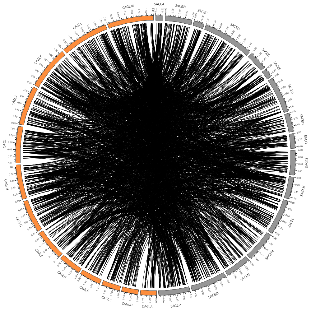
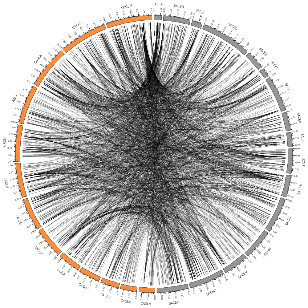
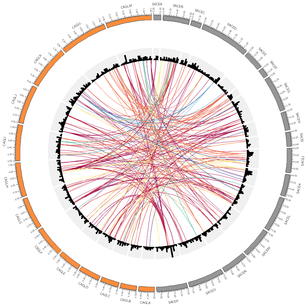
record_limit = 1000 If you drew a lot of links in the previous section, the entire image was saturated with black because all the links overlapped and filled the image.
You can set a color's transparency by using the _aN suffix on the color's name. In the underlying Circos configuration files (which are included at the bottom of this file) I've defined a parameter
auto_alpha_steps = 20
This gives you 20 levels of transparency for each color.
black     -> opaque
black_a1  -> 1/21 transparent
black_a2  -> 2/21 transparent
...
black_a20 -> 20/21 transparent
For obvious reasons, you don't need a 100% transparent version of each color, so the denominator in the fractions above is N+1. If you're interested look in the sessions/day.1/etc directory. If you follow all the include directives up the tree, you'll find that this file is included by all the parts of all the lectures for this day.
color = black_a18
Even with _a18 (85% = 18/21 transparency) the image looks quite busy. Try _a20. In the last lecture, you saw how rules were used to change the color of histogram and heat map bins. In the same way, they can be used to change how links are drawn.
Turn the rules on below by setting use=yes.
<rules>
use = no
Let's remove some links form the image. You discovered in the last section that the minimum size of the start of the links in this top 10,000 set is about 3.4 kb.
Let's only show those that have a size of at least 5 kb.
To do this, we set a condition that triggers for links smaller than 5 kb. Any other directives or parameters in the rule will be applied to these links before they're drawn. In this case setting show=no will hide the links.
size1 is the size of the interval of the start of the link and size2 is the size of its end. Here we're testing whether either of these is smaller than 4kb.
<rule>
condition     = var(size1) < 5000 || var(size2) < 5000
show          = no
</rule>
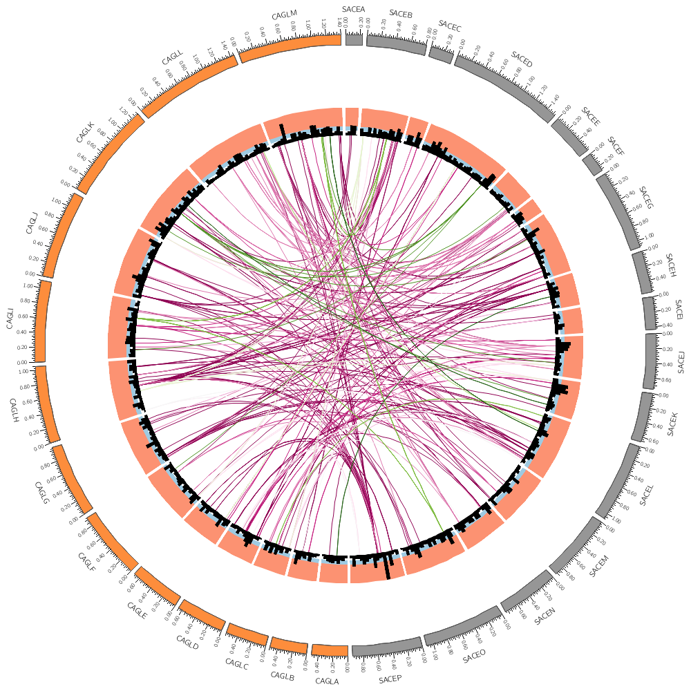
The rule below maps the color of the link based on the size of its start given by var(size1) onto the 11-color diverging spectral Brewer palette. Two additional lines change the thickness of the link and its z-depth.
Circos defines a large number of named colors. All these definitions are in the Circos installation directory under etc/. For convenience, I have included these files in colornames/ in this lecture's section. You'll see the contents of colors.conf below.
<rule>
use           = no
This condition applies to all data points that reach this rule.
condition = 1
The function remap_int(var,min,max,mapmin,mapmax) linearly maps the value given by var from the range [min,max] to [mapmin,mapmax]. We're using sprintf(fmt,list) to format the value as a string that corresponds to the name of a Brewer color.
The eval() is required to parse the contents as code as opposed to treating them as a string literal. Without eval(), z would be set to the literal string "var(size1") and not to the actual value of the size1 parameter.
color         = eval(sprintf("spectral-11-div-%d",remap_int(var(size1),5000,10000,1,11)))
thickness     = eval(sprintf("%d",remap_int(var(size1),5000,10000,1,3)))
The z parameter determines the order in which links are drawn. Links with lower z are drawn before (i.e. below) those with higher z.
z             = eval(var(size1))

</rule>
</rules>

</link>
</links>
RGB color definition. Colors are refered to within configuration files by their name. In order to use a color, you must define it here.
Default triplet is rgb
red = 255,0,0
red = rgb(255,0,0)
You can use LCH and HSV also
red = hsv(0,1,1)
red = lch(54,105,40)
Common colors (red, green, blue, etc) are already defined in 7 tones, based on 7 color Brewer palettes, where available.
vvlHUE (very very light HUE, e.g. vvlred)
vlHUE (very light HUE, e.g. vlred)
lHUE  (light HUE, e.g. red)
HUE   (e.g. red)
dHUE  (dark HUE, e.g. dred)
vdHUE (very dark HUE, e.g. vdred))
vvdHUE (very very dark HUE, e.g. vvdred))
Pure colors are prefixed with "p" (e.g. pred, dpred, vdpred) and are based on 10% luminance steps from a pure hue color. Use these at your discretion.
Boutique colors are not. If you really must use 'bisque', then add
bisque = 255,228,196
See colors.unixnames.txt for a large number of named color definitions.
In addition to hues, two other color groups are defined: (1) Cytogenetic band colors (e.g. gposNNN, acen, stalk, etc.) which correspond to colors on ideogram bands. (2) UCSC chromosome color palette (e.g. chrNN, chrUn, chrNA), included from colors.ucsc.conf.
Another useful list of colors is in colors.brewer.conf, which defines Brewer Palettes, and corresponding lists.
white       = 255,255,255
vvvvlgrey   = greys-9-seq-1
vvvlgrey    = greys-9-seq-1
vvlgrey     = greys-9-seq-2
vlgrey      = greys-9-seq-3
lgrey       = greys-9-seq-4
grey        = greys-9-seq-5
dgrey       = greys-9-seq-6
vdgrey      = greys-9-seq-7
vvdgrey     = greys-9-seq-8
vvvdgrey    = greys-9-seq-9
vvvvdgrey   = greys-9-seq-9
black       = 0,0,0
transparent = 0,0,1

vvlred  = reds-7-seq-1
vlred   = reds-7-seq-2
lred    = reds-7-seq-3
red     = reds-7-seq-4
dred    = reds-7-seq-5
vdred   = reds-7-seq-6
vvdred  = reds-7-seq-7

vvlpred = 255,82,82
vlpred  = 255,63,63
lpred   = 255,41,41
pred    = 255,0,0
dpred   = 237,0,0
vdpred  = 219,0,0
vvdpred = 201,0,0

vvlgreen = greens-7-seq-1
vlgreen  = greens-7-seq-2
lgreen   = greens-7-seq-3
green    = greens-7-seq-4
dgreen   = greens-7-seq-5
vdgreen  = greens-7-seq-6
vvdgreen = greens-7-seq-7

vvlpgreen = 145,255,145
vlpgreen  = 112,255,112
lpgreen   = 75,255,75
pgreen    = 0,255,0
dpgreen   = 0,229,0
vdpgreen  = 0,204,0
vvdpgreen = 0,180,0

vvlblue = blues-7-seq-1
vlblue  = blues-7-seq-2
lblue   = blues-7-seq-3
blue    = blues-7-seq-4
dblue   = blues-7-seq-5
vdblue  = blues-7-seq-6
vvdblue = blues-7-seq-7

vvlpblue = 120,224,250
vlpblue  = 95,206,255
lpblue   = 64,188,255
pblue    = 0,170,255
dpblue   = 0,153,237
vdpblue  = 0,136,220
vvdpblue = 0,120,204

vvlpurple = purples-7-seq-1
vlpurple  = purples-7-seq-2
lpurple   = purples-7-seq-3
purple    = purples-7-seq-4
dpurple   = purples-7-seq-5
vdpurple  = purples-7-seq-6
vvdpurple = purples-7-seq-7

vvlppurple = 166,158,255
vlppurple  = 151,143,255
lppurple   = 136,128,255
ppurple    = 122,112,255
dppurple   = 107,97,243
vdppurple  = 92,80,232
vvdppurple = 77,62,224

vvlorange = oranges-7-seq-1
vlorange  = oranges-7-seq-2
lorange   = oranges-7-seq-3
orange    = oranges-7-seq-4
dorange   = oranges-7-seq-5
vdorange  = oranges-7-seq-6
vvdorange = oranges-7-seq-7

vvlporange = 255,182,106
vlporange  = 255,164,82
lporange   = 255,146,54
porange    = 255,127,0
dporange   = 234,110,0
vdporange  = 213,92,0
vvdporange = 193,75,0
Since there is no sequential yellow Brewer palette, a CMYK-based ladder is used here.
vvlyellow = 255,252,213
vlyellow  = 255,249,174
lyellow   = 255,246,133
yellow    = 255,244,80
dyellow   = 255,242,0
vdyellow  = 227,210,0
vvdyellow = 193,180,0

vvlpyellow = vvlyellow
vlpyellow  = vlyellow
lpyellow   = lyellow
pyellow    = yellow
dpyellow   = dyellow
vdpyellow  = vdyellow
vvdpyellow = vvdyellow
Brewer palettes
<<include colors.brewer.conf>>
UCSC chromosome colors
<<include colors.ucsc.conf>>
HSV pure colors
<<include colors.hsv.conf>>
chromosomes_display_default = no
chromosomes = /sace|cagl/

<links>
<link>
file          = ../../data/links.conservation.10000.txt
radius        = 0.70r
bezier_radius = 0r
thickness     = 1
color         = black_a15

<rules>

<rule>
condition     = var(size1) < 5500
show          = no
</rule>
Try other Brewer palettes here, such as piyg-11-div and reds-11-seq. Make sure you understand how remap_int is working.
<rule>
condition     = 1
color         = eval(sprintf("spectral-11-div-%d",remap_int(var(size1),5500,10000,1,11)))
z             = eval(var(size1))
</rule>

</rules>

</link>
</links>
These are histograms of the counts of the conservation links in 50 kb windows.
<plots>
<plot>
file        = ../../data/links.conservation.count.50kb.txt
type        = histogram
fill_color  = black
stroke_thickness  = 0
r1 = 0.79r
r0 = 0.70r
orientation = out
You can reference the min, max, average (avg), standard deviation (sd) of a track using var(plot_STATISTIC). For example, var(plot_avg) gives the average and the rule above, when activated, fills assigns a black fill to bins whose size smaller than track average.
<rules>
use        = no
<rule>
condition  = var(value) < var(plot_avg)
fill_color = grey
</rule>
</rules>
Use the histogram script to generate a distribution of link counts from the data file used here. What is the 80% percentile count? Change the y0 and y1 values below to (a) color background light red above 80% percentile and (b) color background light blue between 50% and 80% percentile.
<backgrounds>
<background>
color = vvlgrey
y1 = 300 # change this to 80% percentile y0 = 50 # change this to 50% percentile
</background>

</backgrounds>

</plot>

</plots>
chromosomes_display_default = no

chromosomes = /[scz]/ # why does this display all the chromosomes?
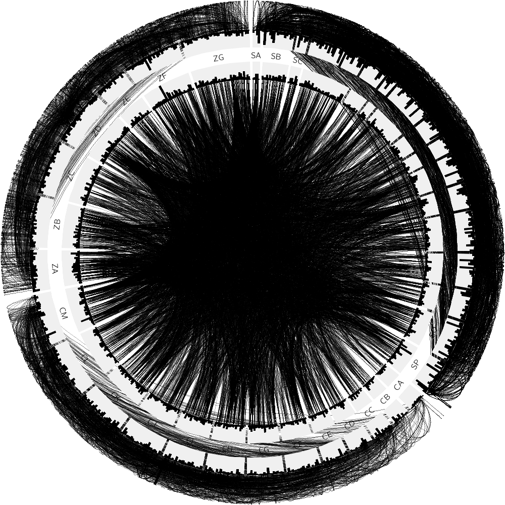
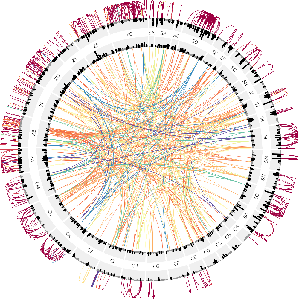
In this section, we'll extend the previous example and add intrachromosomal links, which will be oriented outwards.
<links>

<link>
file          = ../../data/links.conservation.10000.txt
radius        = 0.70r
bezier_radius = 0r
thickness     = 1
color         = black_a15

<rules>
use           = no

<rule>
condition     = var(size1) < 6000
show          = no
</rule>

<rule>
condition     = 1
color         = eval(sprintf("spectral-11-div-%d",remap_int(var(size1),5000,10000,1,11)))
z             = eval(var(size1))

</rule>
</rules>

</link>
If you set the bezier_radius to be larger than the radius, the control point for the link curve will be placed further from the center of the circle than the ends and cause the link to face away from the circle. For more details about link geometry, see Link geometry Circos tutorial.
<link>
file          = ../../data/links.duplication.10000.txt
radius        = 0.90r
bezier_radius = 1.15r
thickness     = 1
color         = black_a15
Create an image without any rules first—what a mess! Activete the rules one by one.
<rules>
use           = no
What does the rule below do?
<rule>
condition     = var(chr1) ne var(chr2) || var(size1) < 4000
show          = no
</rule>

<rule>
condition     = 1
color         = eval(sprintf("spectral-11-div-%d",remap_int(var(size1),5000,10000,1,11)))
z             = eval(var(size1))
</rule>
</rules>

</link>

</links>
These are histograms of the counts of the conservation links in 50 kb windows.
<plots>
<plot>
file        = ../../data/links.conservation.count.50kb.txt
type        = histogram
fill_color  = black
stroke_thickness  = 0
r1 = 0.77r
r0 = 0.70r
orientation = out

<rules>
use = no

<rule>
condition  = var(value) < var(plot_avg)
fill_color = grey
</rule>
</rules>

<backgrounds>
<background>
color = vvlgrey
</background>
</backgrounds>

</plot>

<plot>
file             = ../../data/links.duplication.count.50kb.txt
type             = histogram
fill_color       = black
stroke_thickness = 0
r1 = 0.90r
r0 = 0.83r
orientation = in
You can reference the min, max, average (avg), standard deviation (sd) of a track using var(plot_STATISTIC). For example, var(plot_avg) gives the average and the rule above, when activated, fills assigns a black fill to bins whose size smaller than track average.
<rules>
use = no

<rule>
condition  = var(value) < var(plot_avg)
fill_color = grey
</rule>
</rules>

<backgrounds>
<background>
color = vvlgrey
</background>
</backgrounds>

</plot>

</plots>

<<include ideogram.conf>>
We're not going to show ticks in this image.
<<include ../../../etc/ticks.conf>>
Parameters that control how the ideograms are drawn are defined in a <ideogram> block, which is traditionally stored in ideogram.conf.
<ideogram>
Spacing between ideograms. The r suffix indicates "relative" to the circumference of the circle.
<spacing>
default = 0.0025r
</spacing>
Thickness and color of ideograms. Setting all this to zero will not draw anything.
thickness        = 0p
stroke_thickness = 0
stroke_color     = black
fill             = no
Fractional radius position of chromosome ideogram within image
radius         = 0.98r
show_label     = yes
label_font     = default
label_color    = black
label_radius   = dims(image,radius) - 115p
label_size     = 12
label_parallel = yes
label_case     = upper
Changes the label of each ideogram. Look at the labels and figure out what the code here is doing. You can find documentation to the Perl substr function using perldoc.
perldoc -f substr
label_format   = eval( substr(var(label),0,1) . substr(var(label),-1,1) )

</ideogram>