Learning Circos
Bioinformatics and Genome Analysis
Fondazione Edmund Mach, San Michele all'Adige, Italy, 20 June 2019
v2.00 16 June 2019 Download PDF slides
v2.00 16 June 2019
A 1-day practical course in genomic data visualization with Circos. This material is part of the Bioinformatics and Genome Analysis course held at the Fondazione Edmund Mach in San Michele all'Adige, Italy. Materials also available here: course materials and PDF slides.
Quick links
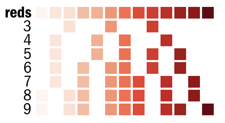
MyPads | BCGA 2019 | 4-day Circos course | Circos documentation best practices getting started | Brewer palettes | Color resources | Nature Methods Points of View Points of Significance
Genomic Data Visualization with Circos
Thursday 20 June 2019 — Day 1
09h00 – 10h30 | Lecture 1 — Introduction to Circos
11h00 – 12h30 | Lecture (practical) 2 — Visualizing gene distribution and size in Yeast—the histogram data track
14h00 – 15h30 | Lecture (practical) 3 — Conservation in Yeast—the link data track
16h00 – 18h00 | Lecture (practical) 4 — Drawing the human genome
18h15 – 19h30 | Lecture (practical) 5 — Afterhours—Perl refresher
18h15 – 19h30 | Lecture (practical) 6 — Afterhours—Visualizing an Ebola strain
Concepts covered today
Circos configuration, common Circos errors, Circos debugging, ideograms, selecting ideograms with regular expressions, input data format, creating Circos data files, data tracks (histograms, heat map, tiles, links), color definitions and using transparency, Brewer palettes, dynamic data formatting rules, downloading files from UCSC genome browser, essential command-line tools and basic scripting,
Visualizing gene distribution and size in Yeast—the histogram data track
Course file structure
This is our first practical session. It will be a brief introduction to Circos, meant to give you a rough overview. We'll get into more details later.
To get started, let's assume that you have the course materials installed in
DIR=~/circos/course
Switch to this lecture lecture
 cd $DIR
 cd sessions/day.1/lecture.2
 ls
You can save this directory as a shell variable using
>export DIR=~/circos/course
at the terminal or add the line to your .bashrc.
You'll want to explore the numbered directories in this lecture's directory
 1/
 2/
 ...
These are stand-alone parts of the lecture. Anything you do within these directories don't impact other parts of this lecture or other lectures.
cd 1/
Within each part you'll find a configuration directory
etc/
that contains the files used to generate the Circos image. This is the configuration and (at times) data files. In some cases, data files are taken from the day's top directory, such as
day.1/data
Creating Circos images from course files
To create the image, just execute 'circos' at the prompt within the lecture's part directory
 > pwd
 ~/circos/course/sessions/day.1/lecture.2/1
 > circos
 debuggroup summary 0.22s welcome to circos v0.69-8 15 Jun 2019 on Perl 5.010000
 ...
 debuggroup output 7.41s created PNG image ./circos.png (229 kb)
Now look at the output image. You may have to refresh your viewer if you're overwriting the image.
Open the configuration file
etc/circos.conf
in an editor and follow the instructions. Sometimes you'll be asked to make changes and regenerate the image. At other times, you'll need to look at data files and write some scripts.
To create an image with a different file name
 > circos -outputfile circos.new.png
 debuggroup summary 0.22s welcome to circos v0.69-8 15 Jun 2019 on Perl 5.010000
 ...
 debuggroup output 7.41s created PNG image ./circos.new.png (229 kb)
In some lecture section directories you'll find circos.final.png. This is the image that you're working towards in that section.
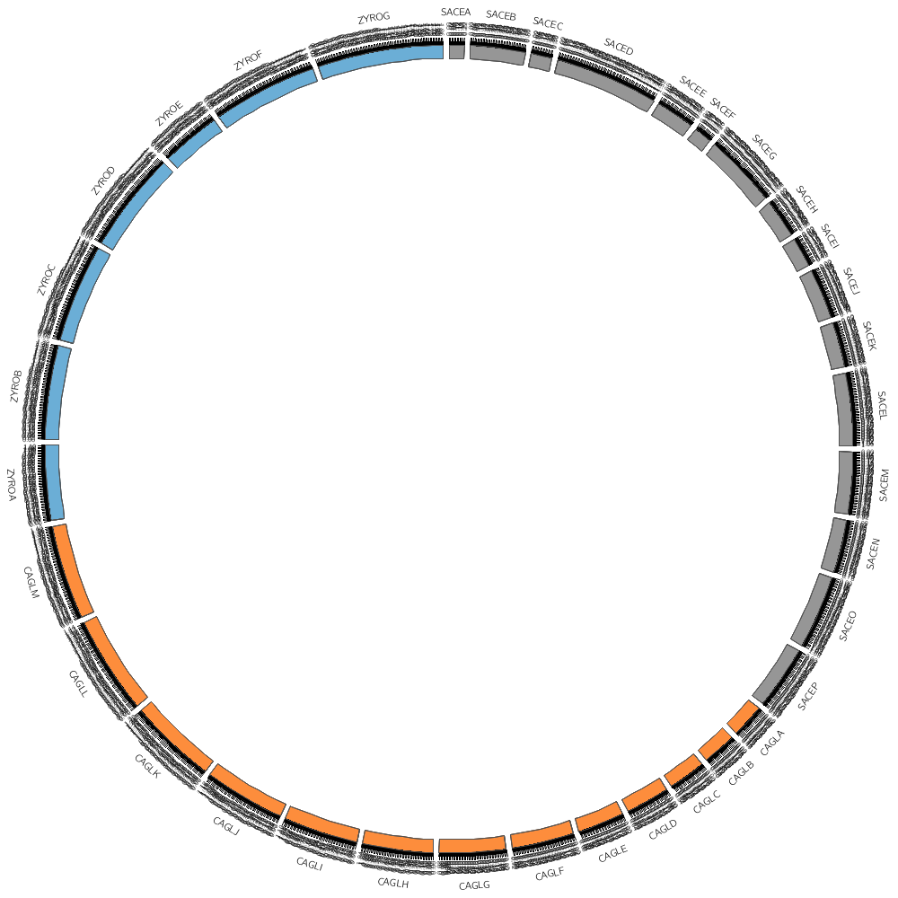
Chromosomes and Ideograms
Central in a Circos figure are the ideograms and their order, scale and orientation.
An ideogram is the graphical depiction of a chromosome and, generally, any stretch of sequence. A chromosome may be shown as a single ideogram, in whole or cropped, or as multiple ideograms, if you divide it into several regions. It is important to create an ideogram layout that helps the reader parse and understand the data.
For example, if you are comparing a single chromosome of one genome (e.g. human chr1) to an entire mammalian genome (e.g. mouse), it is helpful to magnify the human chromosome (e.g. so that it takes 50% of the figure) to present its data at a higher resolution.
On the other hand, if you are comparing two genomes, or roughly equal size subsets of two genomes, it is helpful to scale the ideograms to have the same size to create a pleasing symmetrical layout.
Circos Karyotype file
The karyotype defines all the chromosomes (name, label, length, color)
karyotype = ../../data/karyotype.txt
You will find the karyotype for the three species of yeast you already worked on in the data/ directory two levels up. The relative link allows you to move the course content into any directory (as long as the relative position of the data/ directory relative to the configuration file is unchanged) without having to edit the configuration.
The content of this file is based on data you worked on in the "Large-scale genome comparisons" lectures with Fredj and exactly the same as the Karyotype.tab file you created.
# chr - name label 0 length color

#SACE Saccharomyces cerevisiae
chr - sace-a saceA 0 230218 grey
chr - sace-b saceB 0 813184 grey
chr - sace-c saceC 0 316620 grey
chr - sace-d saceD 0 1531933 grey
chr - sace-e saceE 0 576874 grey
chr - sace-f saceF 0 270161 grey
chr - sace-g saceG 0 1090940 grey
chr - sace-h saceH 0 562643 grey
chr - sace-i saceI 0 439888 grey
chr - sace-j saceJ 0 745751 grey
chr - sace-k saceK 0 666816 grey
chr - sace-l saceL 0 1078177 grey
chr - sace-m saceM 0 924431 grey
chr - sace-n saceN 0 784333 grey
chr - sace-o saceO 0 1091291 grey
chr - sace-p saceP 0 948066 grey

# CAGL Candida glabrata
chr - cagl-a caglA 0 491328 orange
...
chr - cagl-m caglM 0 1402899 orange

ZYRO Zygosaccharomyces rouxii
chr - zyro-a zyroA 0 1114666 blue
...
chr - zyro-g zyroG 0 1865392 blue
Circos Configuration file components
Configuration components that you don't need to worry about right now. These define aspects of the image that will remain unchanged
chromosomes_units = 100

<<include ideogram.conf>>
The ticks and tick labels in this image are very dense. Don't worry about this right now, we'll fix it later.
<<include ../../../etc/ticks.conf>>
<<include ../../../etc/image.conf>>
Low-level definitions
The following files are imported from the Circos distribution directory.
<<include etc/colors_fonts_patterns.conf>>
For example, the file above contains the following.
# etc/colors_fonts_patterns.conf
<colors>
<<include etc/colors.conf>>
</colors>
<fonts>
<<include etc/fonts.conf>>
</fonts>
<patterns>
<<include etc/patterns.conf>>
</patterns>
Each of these files define things like colors (Brewer palettes, color lists, etc), fonts https://www.fontsquirrel.com/fonts/computer-modern">CMU Fonts) and texture patterns. For example etc/colors.conf has definitions like
white   = 255,255,255
grey    = greys-9-seq-5
black   = 0,0,0
red     = reds-7-seq-4
green   = greens-7-seq-4
blue    = blues-7-seq-4
orange  = oranges-7-seq-4
yellow  = 255,244,80
...
Some of the color (e.g. the red family) are defined in terms of Brewer colors. You'll learn more about how colors are defined and how to use them later in this lecture. Low-level settings that hardly ever change (e.g. in etc/housekeeping.conf).
<<include etc/housekeeping.conf>>
Circos Errors
As you're editing the configuration files and creating images, you might come across some errors. Stay calm.
Multiple parameter definitions
Most parameters are expected to be defined only once. For example, if you define chromosomes more than once (because you forgot to comment out a previous definition)
chromosomes    = sace-a
chromosomes    = sace-a;sace-b;sace-c;sace-d
you will see this error
CONFIGURATION FILE ERROR

  Configuration parameter [chromosomes] in parent block [_root] has been defined
  more than once in the block shown above, and has been interpreted as a list.
  This is not allowed. Did you forget to comment out an old value of the
  parameter?
The error messages are detailed and try to help you figure out what's going on.
Mismatched or unterminated blocks
If you do not terminate a block, such as <plots>
 <plots>
 ...
 </plots> # you must have this end tag
you'll see an error like this
CONFIGURATION FILE ERROR

 Error parsing the configuration file. The Config::General module reported the
  error

  Config::General: Block "<plots>" has no EndBlock statement (level: 2, chunk
  4202)!
Basically, if the Config::General module complains about a Block then start hunting for mismatched, mispelled or unterminated blocks. It's very easy to type </plot> when you meant </plots>.
 <plots>
  <plot>
  ...
  </plot>
  <plot>
  ...
  </plot>
 </plot> # oops!
Missing data files
This error indicates that Circos could not find a data file you asked for—check the spelling and location of your file. Circos will try to guess the location of the file relative to several paths (current directory, configuration file directory, Circos installation directory) and will list the directories it checked in.
  *** CIRCOS ERROR ***

      cwd:
      /home/martink/work/circos/course/1day.italy/sessions/day.1/lecture.3/4

      command: /home/martink/bin/circos

  Cannot guess the location of file [../../data/links.conservation.count.txt].
  Tried to look in the following directories
     /home/martink/work/circos/course/1day.italy/sessions/day.1/lecture.3/4/.
     /home/martink/work/circos/course/1day.italy/sessions/day.1/lecture.3/4/etc
     /home/martink/work/circos/course/1day.italy/sessions/day.1/lecture.3/4/data
     /home/martink/work/circos/course/1day.italy/sessions/day.1/lecture.3/4/../.
     ...
karyotype = ../../data/karyotype.txt
We can draw any subset of chromosomes defined in the karyotype file. This is useful if we have multiple genomes defined (as in this case) and we want to show only one genome.
By default, Circos draws all the chromosomes defined in the karyotype file in the order that they appear. Let's change this by setting the default display.
chromosomes_display_default = no
Now we have to define what chromosome to draw.
chromosomes = sace-a # draw the sace-a chromosome
If we want to draw more chromosomes from SACE, just add them to the list
#chromosomes = sace-a;sace-b;sace-c;sace-d # a list of chromosomes
But what if we wanted to draw all the SACE chromosomes but didn't really want to have to list them all. For this, use a regular expression.
#chromosomes = /sace/ # regular expression that matches any chromosome with sace substring
There are 36 chromosomes in the karotype file
sace-a ... sace-p
cagl-a ... cagl-m
zyro-a ... zyro-g
Regular expressions are very powerful in matching strings and you should learn their syntax as soon as possible. In fact, why not learn the basics during lunch—I promise you that your life will never be the same (in a good way) after you know their basics.
#chromosomes    = /-a/     # all -a chromosomes
#chromosomes    = /-[abc]/ # all -a, -b or -c chromosomes
By default, all ideograms are drawn in the order that their chromosomes appear in the karyotype file. You can rearrange the order in which ideograms are drawn using chromosomes_order.
For example, we can specify the order of all the -a chromosomes
#chromosomes_order = zyro-a,sace-a,cagl-a
If you have a large number of ideograms and want to put some first, use the caret, ^, to indicate the start of the list and then list the chromosomes to come first. Any that are not mentioned will be drawn after in default order. The ^ character reflects regular expression syntax, where it is used as a an anchor for the start of the string.
For example, if you're drawing all the -a, -b and -c chromosomes, and want zyro-c, sace-b and cagl-c to come first, use
#chromosomes_order = ^,zyro-c,sace-b,cagl-c
This is very helpful when you're displaying images with links and you would like to emphasize one (or more) chromosomes by putting them first. Keep this in mind when we get to drawing more complex images.
Creating Circos data files
You'll find all the Circos data files in day.1/data. These are based on the conservation and duplication data files that you have already generated, which are in day.1/data/conservation and day.1/data/duplication.
These Circos data files are created by day.1/data/create.yeast.tracks, which you should familiarize yourself with this script, especially the bash for loops, variable interpolation and multiplication.
To run this script, you need to be in the day.1/data directory.
 cd ../../data
 ./create.yeast.tracks
The following files are created
genes.txt
genes.count.100kb.txt
genes.count.50kb.txt
genes.count.20kb.txt
genes.count.10kb.txt
genes.count.5kb.txt
genes.avgsize.100kb.txt
genes.avgsize.50kb.txt
genes.avgsize.20kb.txt
genes.avgsize.10kb.txt
genes.avgsize.5kb.txt

links.duplication.txt
links.duplication.10000.txt
links.duplication.count.100kb.txt
links.duplication.count.50kb.txt
links.duplication.count.20kb.txt
links.duplication.count.10kb.txt
links.duplication.count.5kb.txt

links.conservation.txt
links.conservation.10000.txt
links.conservation.count.100kb.txt
links.conservation.count.50kb.txt
links.conservation.count.20kb.txt
links.conservation.count.10kb.txt
links.conservation.count.5kb.txt
#!/bin/bash

# Run this from day.1/data

DATA=.
SCRIPTS=../../scripts

# Change this to the directory where Circos is installed
CIRCOS=/home/martink/work/circos/svn/

echo "Creating list of 16,000 genes"
cat conservation/coords.txt | awk '{print $2,$3,$4,$4-$3+1,"name="$1}' > genes.txt

BINS="5 10 20 50 100"

for ws in $BINS; do
  echo "Counting genes in $ws kb bins"
  bin=$((ws * 1000))
  cat genes.txt | ~/work/circos/svn/tools/resample/bin/resample -bin $bin -count > genes.count.${ws}kb.txt
done

for ws in $BINS; do
  bin=$((ws * 1000))
  echo "Counting genes in $ws kb bins"
  cat genes.txt | $CIRCOS/tools/resample/bin/resample -bin $bin -count > genes.count.${ws}kb.txt
  echo "Calculating gene average size in $ws kb bins"
  cat genes.txt | $CIRCOS/tools/resample/bin/resample -bin $bin -avg > genes.avgsize.${ws}kb.txt
done

for type in conservation duplication; do
  echo "Creating $type links"
  cat $type/C* $type/S* $type/Z* | $SCRIPTS/create.yeast.links -coord $type/coords.txt > links.$type.txt
  echo "...extracting largest 10,000 links"
  N=10000
  cat links.$type.txt | awk '{print $3-$2+1,$0}' | sort -nr | head -$N | cut -d " " -f 2- > links.$type.$N.txt

  for ws in $BINS; do
      bin=$((ws * 1000))
      echo "...counting links in $ws kb bins"
      cat links.$type.txt | $CIRCOS/tools/binlinks/bin/binlinks -bin $bin -num > links.$type.count.${ws}kb.txt
  done

done
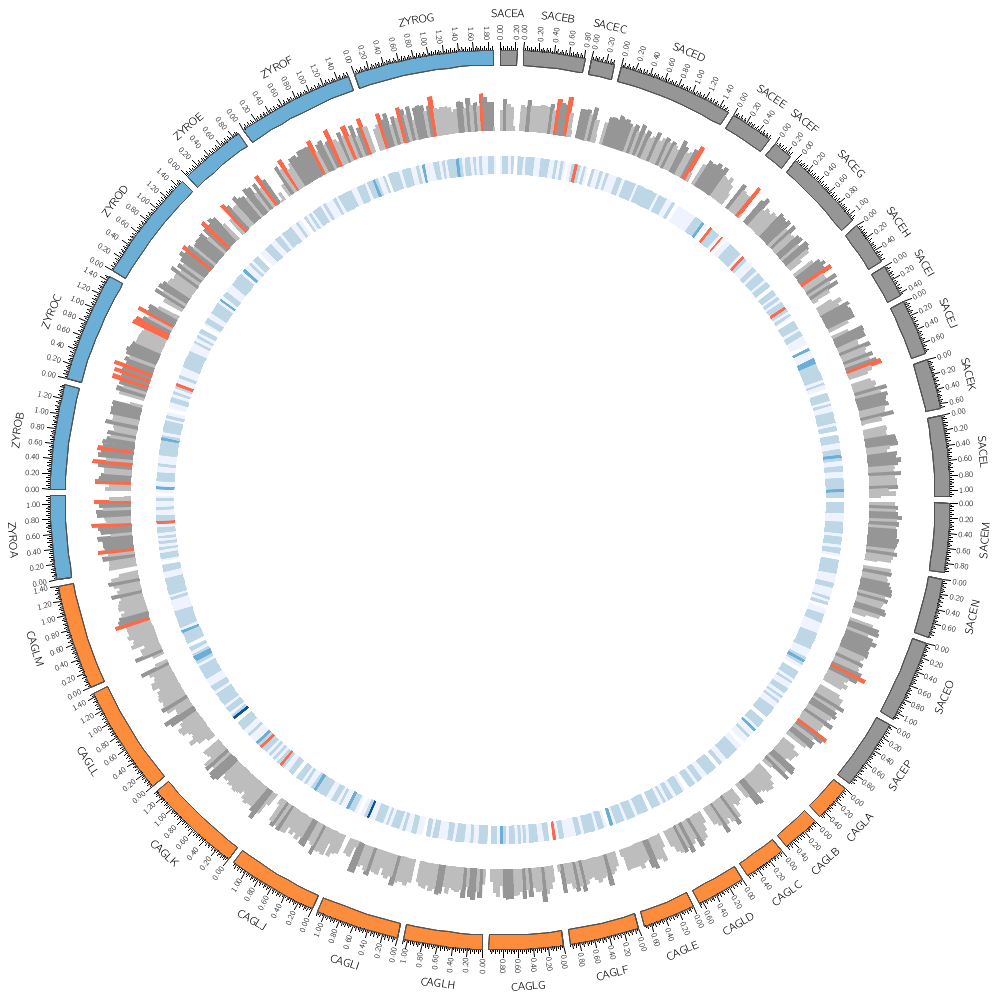
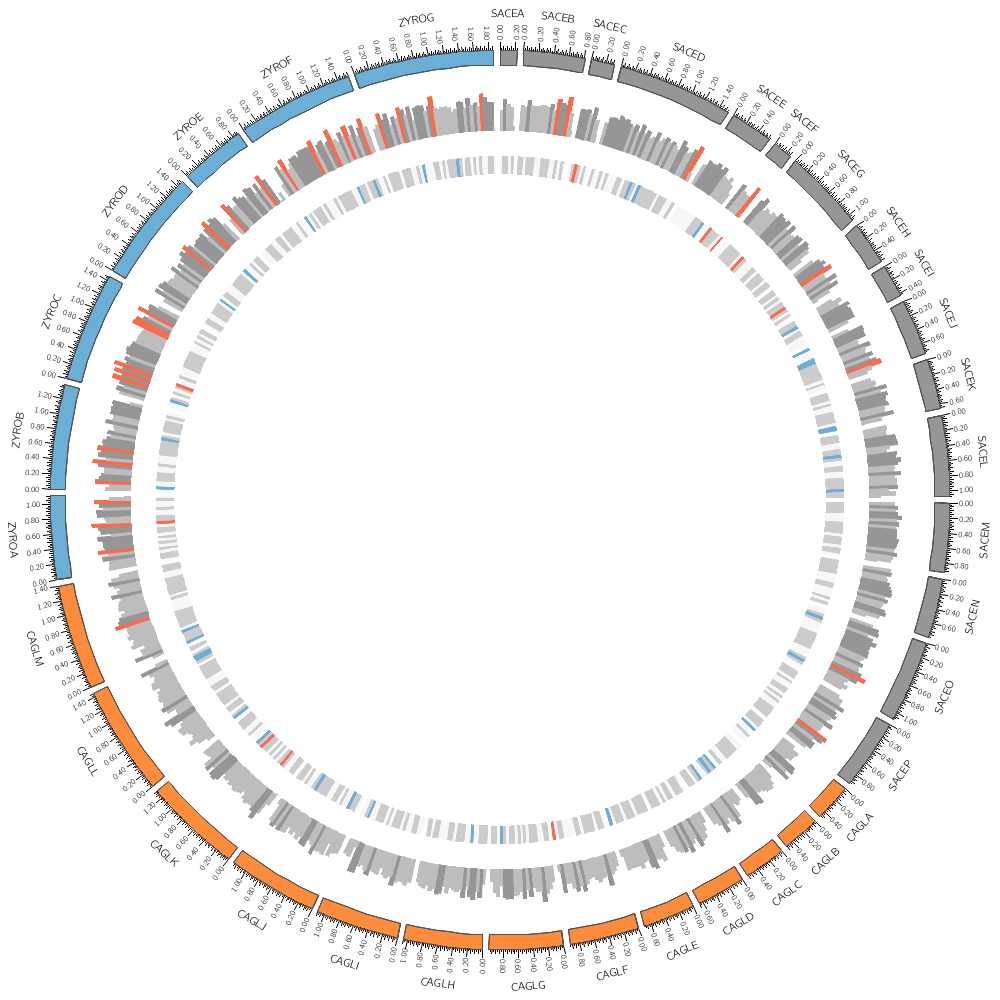
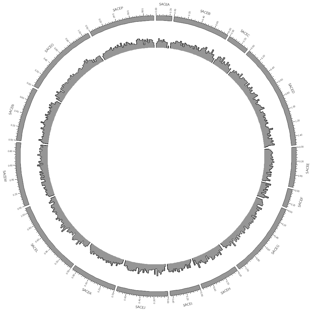
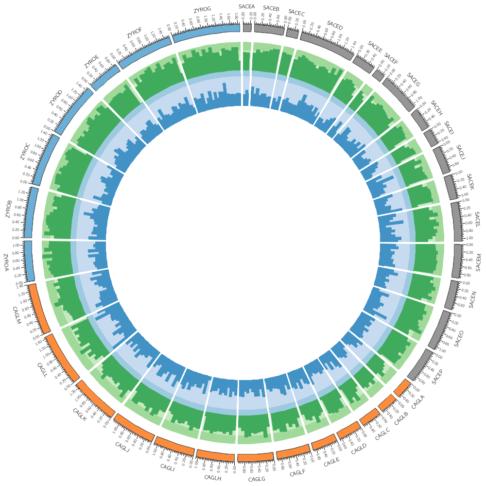
It's time to draw some data! We'll stick with Saccharomyces cerevisiae (SACE) for now.
karyotype = ../../data/karyotype.txt

chromosomes_display_default = no
chromosomes                 = /sace/
Data tracks are defined in <plot> blocks inside an outer <plots> block Let's plot the gene count.
<plots>
<plot>
file       = ../../data/genes.count.20kb.txt
type       = histogram
fill_color = grey
color      = black
stroke_thickness = 1
The format of the data file is
CHR START STOP VALUE
sace-a 0 19999 6
sace-a 20000 39999 8
sace-a 40000 59999 12
sace-a 60000 79999 9
sace-a 80000 99999 10
sace-a 100000 119999 8
...
In this case, the counts are binned into 20 kb regions. Typically, you'll need to parse your data into this format or extract the relevant columns. The location of the track is defined by r0 (inner radius) and r1 (outer radius). They are best expressed as a relative fraction of the ideogram radius. r1 = 0.9r # track ends at 90% of ideogram radius r0 = 0.7r # track starts at 70% of ideogram radius By default the histogram plot points outward but you can flip it with orientation
#orientation = in # in,out
By default the histogram stroke is placed only on the outside. To add a stroke to each individual bin use stroke_type
#stroke_type = both # both,outline

</plot>  # don't forget the closing tag
Now let's add another plot. We'll also plot the average gene size. Notice that use = no in this plot — this turns the plot off. To turn it on, set use = yes or just comment out use = no.
<plot>
use              = no # no,yes
file             = ../../data/genes.avgsize.10kb.txt
type             = histogram
fill_color       = blue
stroke_thickness = 0

r1 = 0.7r
r0 = 0.5r

#orientation = out # out by default

</plot>

</plots>
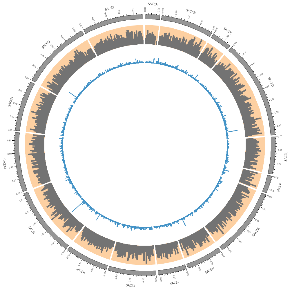
karyotype = ../../data/karyotype.txt

chromosomes_display_default = no
chromosomes                 = /sace/

<plots>
<plot>
file        = ../../data/genes.count.20kb.txt
type        = histogram
fill_color  = dgrey
stroke_thickness  = 0
r1 = 0.95r
r0 = 0.80r
Backgrounds are defined in their own blocks. If you have a single <background> block then by default the background will fill the track.
<backgrounds>
<background>
color = vlorange
</background>
Multiple backgrounds are layered. This one is turned off (use=no) so turn it back on.
<background>
use   = no
color = lorange
y0    = 0.75r   # starts at 75% from bottom of plot
</background>
</backgrounds>
</plot>

<plot>
file             = ../../data/genes.avgsize.10kb.txt
type             = histogram
fill_color       = dblue
stroke_thickness = 0
r1 = 0.79r
r0 = 0.65r

<backgrounds>
use   = no     # use is inherited by all children blocks
<background>
color = vlblue
</background>
<background>
color = lblue
y1    = 5000   # absolute value of end of background
y0    = 2500   # absolute value of start of background
</background>
</backgrounds>

</plot>

</plots>
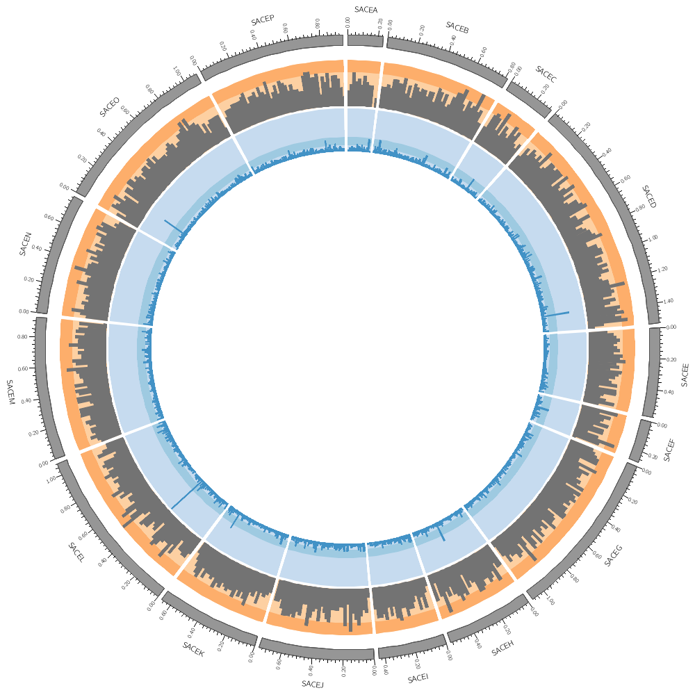
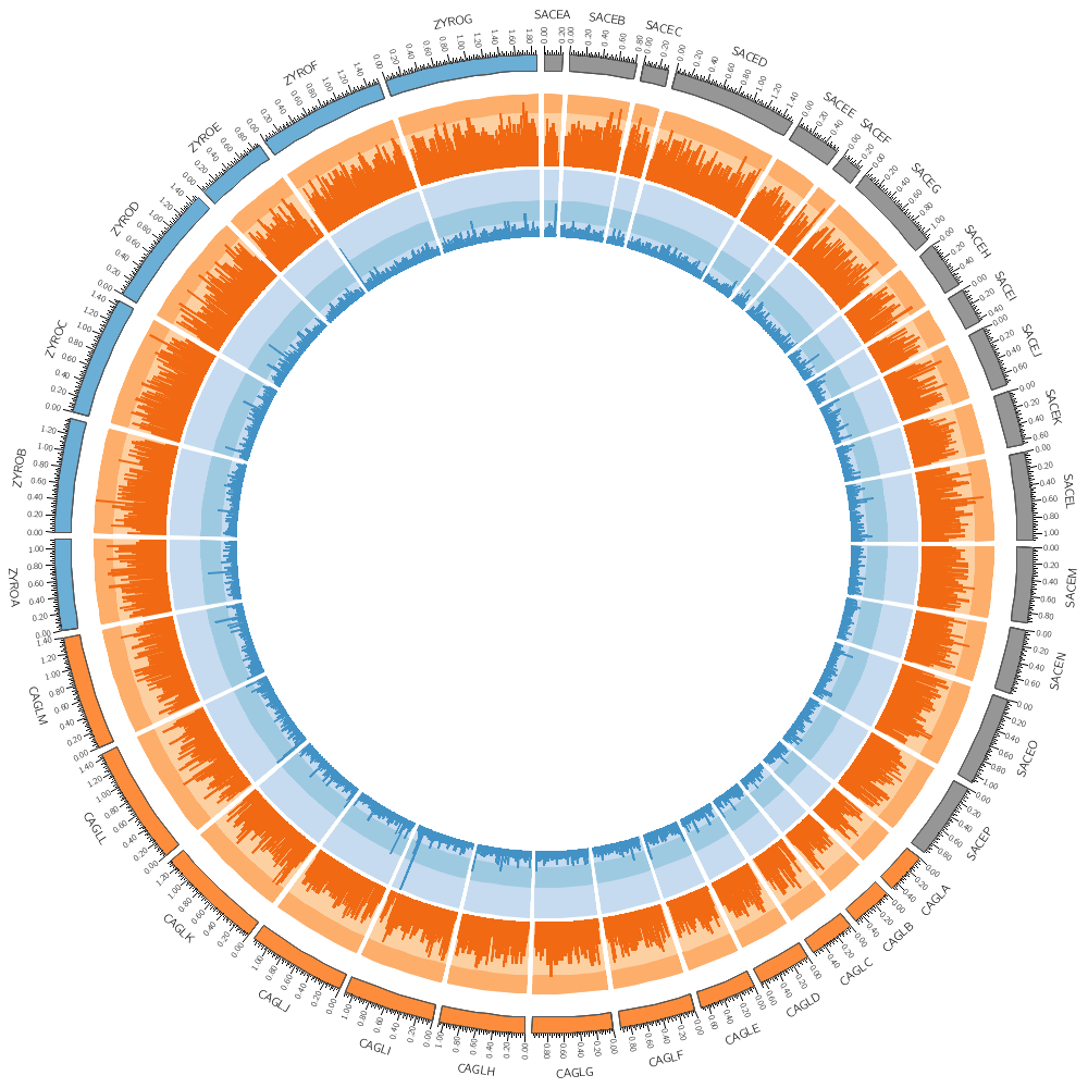
karyotype = ../../data/karyotype.txt
Let's draw all three genomes: SACE, CAGL and ZYRO
chromosomes_display_default = yes
Our data was binned into 20 kb bins for the gene count and 10 kb bins for gene average size. You'll notice that when you run Circos, it tells you that the total size of all chromosomes is 34 Mb.
...
karyotype has 36 chromosomes of total size 34,154,242
...
This means that we have about 3,400 bins for the gene size histogram and 1,700 bins for the gene count histogram. Because we have so many bins, they're thin and hard to see.
You have gene tracks binned into 5, 10, 20, 50 and 100 kb. Create images using the 20, 50 and 100 kb bin tracks. Which looks better?
To learn about visual acuity and guidelines for controlling the size of elements on the screen or page, see
handout/visual.acuity.points.pdf
For background reading about managing resolution for print, see
handout/figure.size.resolution.pdf
I will have a printed copy of both of these handouts — it is important that you see what different size elements and type look like on paper.
<plots>
<plot>
file        = ../../data/genes.count.20kb.txt
type        = histogram
fill_color  = dorange
stroke_thickness  = 0
r1 = 0.95r
r0 = 0.80r
orientation = out
The orange of the track is the same color as the CAGL chromosomes. Using the same color in a figure to encode different things isn't a good idea. Change the orange in this track to green (e.g. dgreen, lgreen, etc)).
<backgrounds>
<background>
color = vlorange
</background>
<background>
color = lorange
y0    = 0.75r
</background>
</backgrounds>
</plot>

<plot>
file             = ../../data/genes.avgsize.20kb.txt
type             = histogram
fill_color       = dblue
stroke_thickness = 0
r1 = 0.79r
r0 = 0.65r
orientation = out
<backgrounds>
<background>
color = vlblue
</background>
<background>
color = lblue
y1    = 5000
y0    = 2500
</background>
</backgrounds>

</plot>

</plots>
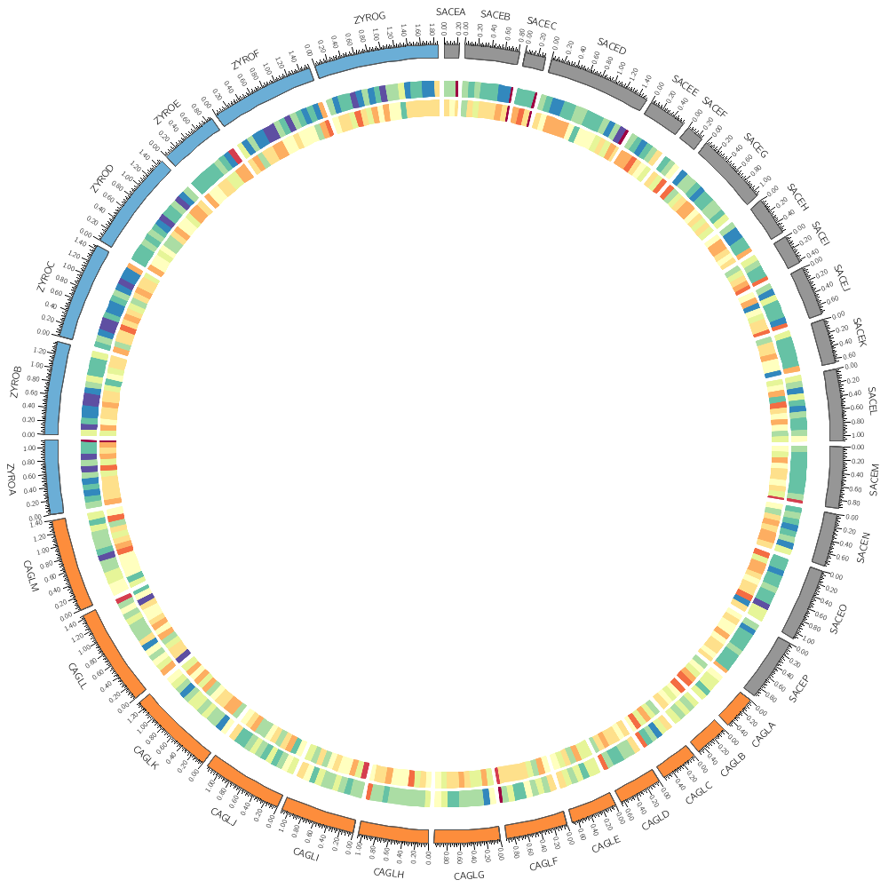
karyotype = ../../data/karyotype.txt

chromosomes_display_default = yes

# In addition to histograms, you can draw scatter plots, line plots,
# heat maps and other 2-dimensional data encodings.
#
# Most of these use exactly the same file format. To change how data
# is displayed, all you need to do is change the type
# field.
#
# Sometimes, a few other parameters that are specific to this
# encoding will need to be changed.  However, there are sensible
# defaults for each encoding type.
#
# Instead of a histogram, let's draw the gene count and size as a heat map.

# But first, let's define the bin size to be used later in the file.

bin_size = 100kb # files are available for 5kb 10kb 20kb 50kb 100kb

<plots>
<plot>

# Let's use the data file from the previous part of this lecture. We can refer to the
# bin_size parameter using conf(bin_size).

file        = ../../data/genes.count.conf(bin_size).txt
type        = heatmap
r1 = 0.94r
r0 = 0.90r
</plot>

<plot>
file             = ../../data/genes.avgsize.conf(bin_size).txt
type             = heatmap
r1 = 0.89r
r0 = 0.85r
</plot>

# Change the bin_size definition to 50kb and replot the figure. See
# how the heat map elements are now half the size and are starting to
# get harder to distinguish.

# If multiple <plot> blocks are using the same parameters, you can
# define the parameters in the <plots> block and take advantage of
# inheritance. Anything that is defined in <plots> is inherited by
# <plot>, unless it is overridden.

file             = ../../data/genes.avgsize.conf(bin_size).txt
type             = heatmap

# Each of the three blocks below will use the same value of file and type,
# as defined above. The first two <plot> blocks above also inherit this,
# but they have their own overriding values.
#
# By default, heatmaps use the Brewer spectral palette. Turn on the
# blocks below and see how the previous track looks like using
# 5-color sequential grey palette (greys-5), the 7-color sequential
# blue palette (blues-7) and the 9-color diverging pink-yellow-green
# palette (piyg-9).

<plot>
use = no
r1 = 0.84r
r0 = 0.80r
color = greys-5
</plot>

<plot>
use = no
r1 = 0.79r
r0 = 0.75r
color = blues-7
</plot>

<plot>
use = no
r1 = 0.74r
r0 = 0.70r
color = piyg-9
</plot>

# Typically, for each palette you have 3 to 11 color versions available.
# Define a global num_colors parameter, set it to 11, and then edit the
# plots above to reference this parameter the same way as bin_size was
# referenced in the previous blocks.
#
# Try 7, 9 and 11 colors — is there benefit to more colors?
#
# For all the Brewer palettes, see handouts/brewer-palette-swatches.pdf

</plots>
Below, I show you a part of the Circos configuration file that defines the Brewer palette colors. You can find this file in etc/colors.brewer.conf in the Circos installation directory.
Colors from www.colorbrewer.org by Cynthia A. Brewer,
Geography, Pennsylvania State University. See BREWER for license.
Color names are palette-numcolors-type-idx (e.g. reds-3-seq-1)
palette   palette name (e.g. reds)
numcolors number of colors in the palette (e.g. 3)
type      palette type (div, seq, qual)
idx       color index within the palette (e.g. 1)
Another version of the color index is defined where colorcode is the color's letter unique to a given palette.
For each palette, two color list are defined for use with heatmaps.
palette-numcolors-type
palette-numcolors-type-rev
where the second contains colors in reversed order.
Also supported is the format
palette-numcolors
palette-numcolors-rev
(without the -type), which isn't necessary to uniquely identify the palette.
Each diverging and sequential palette has all the colors used for its n-color variants listed an integrated 13-color (for sequential) or 15-color (for diverging) palettes.
http://www.personal.psu.edu/cab38/ColorBrewer/ColorBrewer_updates.html
http://mkweb.bcgsc.ca/brewer
For example, the 3-color sequential blues palette is defined by these colors
blues-3-seq = blues-3-seq-(\d+)
blues-3-seq-rev = rev(blues-3-seq-(\d+))
blues-3-seq-1 = 222,235,247
blues-3-seq-2 = 158,202,225
blues-3-seq-3 = 49,130,189
And the 4-color version of it is
blues-4-seq = blues-4-seq-(\d+)
blues-4-seq-rev = rev(blues-4-seq-(\d+))
blues-4-seq-1 = 239,243,255
blues-4-seq-2 = 189,215,231
blues-4-seq-3 = 107,174,214
blues-4-seq-4 = 33,113,181
Here is the 11-color spectral palette
spectral-11-div = spectral-11-div-(\d+)
spectral-11-div-rev = rev(spectral-11-div-(\d+))
spectral-11-div-1 = 158,1,66
spectral-11-div-2 = 213,62,79
spectral-11-div-3 = 244,109,67
spectral-11-div-4 = 253,174,97
spectral-11-div-5 = 254,224,139
spectral-11-div-6 = 255,255,191
spectral-11-div-7 = 230,245,152
spectral-11-div-8 = 171,221,164
spectral-11-div-9 = 102,194,165
spectral-11-div-10 = 50,136,189
spectral-11-div-11 = 94,79,162
spectral-15-div-11 = 153,213,148
spectral-11 = spectral-11-div-(\d+)
spectral-11-rev = rev(spectral-11-div-(\d+))
Some tracks such as the heat maps, which map values to colors automatically, take the name of a color list, in which case you would put the name of the palette without color index
color = spectral-11-div
In most cases though you'll be refering to specific colors
color = spectral-11-div-7
bin_size = 50kb
Let's return to the histogram and heatmap.
You can change how data is displayed (any data point, such as a histogram bar, heat map bin, etc) based on conditions, which can be a function of the data value, position and other property of the data point or track.
For example, you can hide data points that are
- on specific chromosomes - at specific positions or within intervals - that are smaller, greater than, or within a value range
or any combination of these. You can mix in Perl code into the condition, too.
You could add this formatting to the input file. For example, if you wanted to make a specific histogram bin have a red fill color, you can include it as an optional column
sace-a 0 19999 6
sace-a 20000 39999 8 fill_color=grey
sace-a 40000 59999 12 fill_color=red
sace-a 60000 79999 9
This might make sense if the decision to change the color was very complicated. But if the condition is relatively straightforward (such as the kind listed above), it's better practise to store the formatting separately from the data.
<plots>
<plot>

file        = ../../data/genes.count.conf(bin_size).txt
type        = histogram
fill_color  = grey
stroke_thickness = 0
r1 = 0.94r
r0 = 0.85r
Rules are defined in a <rules> block within a <plot> block. Each plot has its own rules. Individual rules are in a <rule> block.
Make sure that you place these inside a <plot> block.
A rule has a condition. If it evaluates to true then any parameters defined in the rule are applied to the data point.
Rules are evaluated in the order that they appear in the <rules> block and applied to each data point independently. As soon as a rule is applied to a data point, no more rules are tested for that data point (unless you explicitly ask for this). If you want to continue testing other rules after a rule has been triggered, you have to include
flow = continue
in the rule from which you wish to continue. We'll see this later.
<rules>
This rule will apply a light grey fill to any bins whose value is less than 25.
<rule>
condition  = var(value) < 25
fill_color = lgrey
</rule>
Add a rule that turns all points with value larger than 30 to red.
<rule>
condition  = var(value) > 30
fill_color = red
</rule>

</rules>
</plot>

<plot>
file        = ../../data/genes.avgsize.conf(bin_size).txt
type        = heatmap
color       = blues-5
r1 = 0.79r
r0 = 0.75r

<rules>
This rule will hide any heat map bins whose value is less than 750
<rule>
condition  = var(value) < 750
show       = no
</rule>
Any bins whose value is in the range (1000,1100) will be red.
<rule>
condition  = var(value) > 1000 && var(value) < 1100
color      = red
</rule>
Change the heatmap palette to greys-5 and add a rule that turns all points with value larger than 1500 blue.
</rules>
What other kind of rules do you think might be useful in a heatmap? To help you write rules, try using var(?) in the condition of one of the rules above. When Circos gets to this condition for the first data point, it will report all the variables that are available to you and quit.
You asked for help in the expression [var(?) < 750].
In this expression the arguments marked with * are available for the var() function.

chr * cagl-a
end * 49999
i * 0
next_value * 1875.75
plot_average * 1539.3852433042
plot_avg * 1539.3852433042
plot_max * 3921.42857142857
plot_mean * 1539.3852433042
plot_min * 815.56
plot_n * 694
plot_sd * 283.27981252657
plot_stddev * 283.27981252657
plot_var * 80247.4521850886
rev * 0
start * 0
value * 1635.21428571429
</plot>

</plots>