Have ideas? Tell me.
the best layout
Partially optimized QWKRFY and fully optimized QGMLWY layouts are the last word in easier typing.
the worst layout
A fully anti-optimized TNWMLC layout is a joke and a nightmare. It's also the only keyboard layout that has its own fashion line.
download and explore
Download keyboard layouts, or run the code yourself to explore new layouts. Carpalx is licensed under CC BY-NC-SA 4.0.
layouts
Download and install the layouts.
Simulated Annealing
Stochastic Optimization
Stochastic methods are used when it is very difficult, or impossible, to analytically (or deterministically) find the "best solution" to a problem. These kinds of problems are called np-complete (or np-hard) — you must examine all solutions in order to be assured of having found the best solution.
Identifying all potential solutions to a problem is not practical, except for the simplest problems. If you consider something like a keyboard layout for a keyboard with only 26 keys, it quickly becomes apparent that exploring all potential layouts (`26! = 4\times 10^{26}`) is not feasible. However, the problem is made tractable by the fact that given two layouts you can determine which of the two is better. Moreover, if you think about it a little bit you can probably come up with some kind of number which quantifies the fitness of a given layout. In your search for the best layout, you would examine a variety of layouts and consider only those that had the best fitness.
The 'stochastic' part of the optimization represents the use of random numbers in the process of finding the best layout. Randomness is used to generate new layouts based on the last best solution. Randomness is also used to determine whether a candidate solution is to be accepted (read below). The optimization is therefore not deterministic (it doesn't always give you the same solution, as long as the seed to the random number generator is different).
Usually multiple runs of the simulation are necessary to explore the family of solutions to identify the best one because the phase space of solutions is generally complicated and many local minima exist.
Simulated Annealing
Simulated annealing is one of many types of stochastic optimization algorithms. Because simulated annealing has its roots in physics, the quantity that measures a solution's fitness is frequently referred to as the energy. The algorithm's role is to therefore find the solution for which the energy is minimum. The process of finding this solution begins with starting with some initial guess, which is frequently a random state.
For example, you would start with a keyboard layout on which the keys are randomly organized. Since each potential solution has an associated energy, you compute the energy (`E_0`) and set this value aside. Next, you adjust the solution slightly to obtain a marginally different solution. The size of this adjustment is crucial. If the step is too small, it make take forever to move to a significantly different state. If the step is too large, you risk jumping about the solution space so quickly that you will not converge to a solution. In the case of the keyboard, a reasonable step from one solution to another is a single or double keys swap. Once the new solution has been derived, you compute its energy (`E_1`).
Now that you have `E_0` and `E_1` is where things get interesting. Let `\Delta E = E_1 - E_0`. You might suppose that if `\Delta E < 0` then you should value the new solution over the old one, since its energy is lower. You'd be right — in this case, simulated annealing transitions to the new solution and continues from there. Let's skip over the `\Delta E = 0` case for now. What about when `\Delta E > 0`? In this case, the new solution is less desirable than the old one, since its energy is higher. Do we discard the new solution? Let's consider what would happen if we did.
If all transitions with `\Delta E > 0` are rejected, the algorithm will be greedy and descend towards the lowest-energy solution in the vicinity of the current state. If the step from one solution to another is small, then a minimum energy state will be found. However, this may be a local minimum instead of a global one. If all paths from the local minimum to the global minimum involve an increase in energy (imagine the local minimum being a trough), these paths will never be explored. To mitigate this, and this is where the "stochastic" part of simulated annealing comes into play, the algorithm probabilistically accepts transitions associated with `\Delta E > 0` according to the following probability $$p(\Delta E) \sim \exp(-\Delta E/T)$$
where `\Delta E` is the energy difference and `T` is a parameter that is interpreted as a temperature. The basis for this interpretation originates from the original motivation for the form of the transition probability.
Given a candidate transition and `\Delta E > 0`, the algorithm samples a uniformly distributed random number `r` in the range `[0,1)` and if `r < p`, then performs the transition and accepts the higher energy state. If `\Delta E` is very large, `p` is small and this transition does not happen frequently. If `\Delta E` is small, then this transition is more frequent. $$r = \text{URD}([0,1)) \;\; \begin{cases} r < p(\Delta E), & \text{accept transition} \\r \ge p(\Delta E), & \text{reject transition} \end{cases} $$
The role of the parameter `T` is very important in the probability equation. This parameter is continuously adjusted during the simulation (typically monotonically decreased). The manner in which this parameter is adjusted is called the cooling schedule, again with the interpration of `T` as a temperature. Initially, `T` is large thereby allowing transitions with a large `\Delta E` to be accepted. As the simulation progresses, `T` is made smaller, thereby reducing the size of excursion in to higher energy solutions. Towards the end of the simulation, `T` is very small and transitions with only very slight increases in `E` are allowed.
In carpalx, `T` is cooled exponentially as a function of the iteration, `i`. $$ \begin{array}{rl} T_i =&T_0 \exp{-ik/N} \\p(\Delta E,i) =&p_0 \exp(-\Delta E/T_i) \end{array} $$
The exponential form of `T_i` has nothing to do with the exponential form of the transition probability. It's just a cooling schedule that I selected (admittedly without testing any other form).
The effect of the cooling schedule is to allow the algorithm freedom of movement throughout the solution space at first (large `T`), then progressively converge to a solution with a minimum (medium `T`) and converge to a minimum (small `T`). The optimization simulation is typically run many times, each time with a different starting state.
Parameter Values
Choosing values for `p_0`, `T_0`, `k` and `N` should be done carefully. The possible range of values for `E` must be anticipated and `T` will need to be scaled appropriately to produce useful probability values.
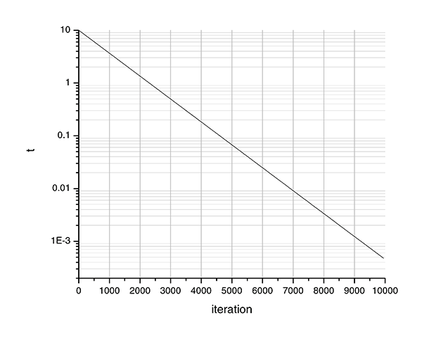
For carpalx, the typing effort ranges from `9` (QWERTY, mod_01) to about `4.5-5` (optimized, mod_01). Consequently, I have chosen the parameters as follows
- `T_0 = 10`
- `k = 10`
`T_0` scales the temperature so that at maximum energy, `E/T` is approximately `1`. With a value of `k=10`, the temperature drops by `1/e` for every 1/10th of the simulation. Initially, the temperature is `T_0 = 10`. At `i=1000`, (10% into the simulation), `T_{1000} = 10/e`. At `i=2000`, (20% into the simulation), `T_{2000} = 10/e^2`, and so on. At the end of the simulation, `T_\text{end} = 10/e^{10} = 4.5\times 10^{-4}`. If you want the temperature to drop faster, use a larger value of `k`. To start with a cooler system, set a lower `T_0`.
For all simulations, I've used
- `p_0 = 1`
- `N = 10000`
References
Metropolis,N., A. Rosenbluth, M. Rosenbluth, A. Teller, E. Teller,
"Equation of State Calculations by Fast Computing Machines",
J. Chem. Phys.,21, 6, 1087-1092, 1953.
The canonical reference on Monte Carlo simulations.
Kirkpatrick, S., C. D. Gelatt Jr., M. P. Vecchi, "Optimization by
Simulated Annealing",Science, 220, 4598, 671-680, 1983.
The canonical reference for simulated annealing.
Cerny, V., "Thermodynamical Approach to the Traveling Salesman
Problem: An Efficient Simulation Algorithm", J. Opt. Theory Appl., 45,
1, 41-51, 1985
Application of simulated annealing to traveling salesman problem.
Metropolis,
Monte Carlo and the MANIAC.
Fun article.