Monday 10 December 2018 — Day 1

9h00 - 10h30 | Lecture 1 — Introduction to Circos

11h00 - 12h30 | Lecture (practical) 2 — Visualizing gene distribution and size in Yeast: the histogram data track

14h00 - 15h30 | Lecture (practical) 3 — Conservation in Yeast: the link data track

16h00 - 18h00 | Lecture (practical) 4 — Visualizing an Ebola strain

Let's draw chromosomes from a couple of the genomes, SACE and CAGL.

Here the regular expression is using the alternation pipe, meaning that chromosome names can match either "sace" or "cagl"

chromosomes_display_default = no
chromosomes = /sace|cagl/

Like plots, links are defined in blocks. Unlike plots, they belong in <links> blocks. Each link track has its own <link> block.

<links>
<link>
file          = ../../data/link_cagl_sace.txt

Different block types expect different parameters. For the links, you need to define the position of the ends of the links. This is best done relative to the ideogram of the circle.

So here our links will go as far as 98% of the radius of the ideogram circle.

radius        = 0.98r

This controls how curved the links are. Specifically, this is the radius of the control point. Try setting this to a larger value like 0.25r or 0.5r.

bezier_radius = 0r

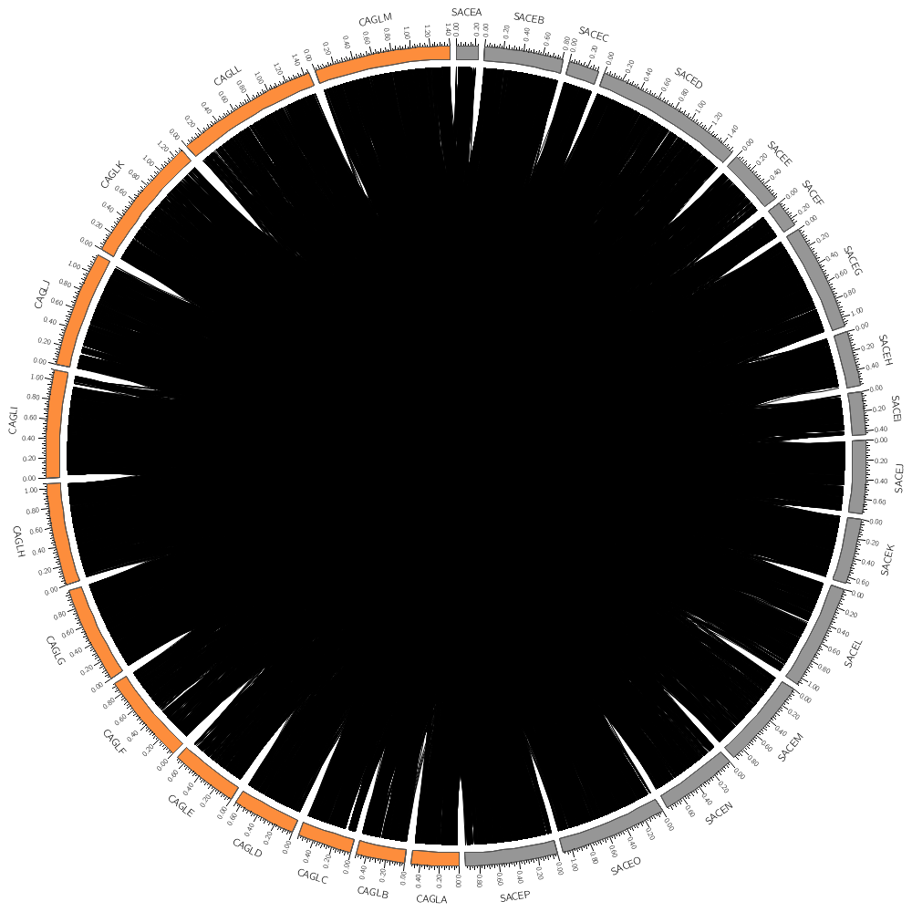
Since there are about 10,000 links in the file, the image might take a while to draw. The record_limit parameter is useful for limiting the number of entries read from the file for debugging. Once you're happy, comment out this line to draw all the links, which may take 20-30 seconds.

#record_limit  = 1000

color         = black
thickness     = 1

</link>
</links>

Since we'll always be using this karyotype file for today, for the rest of today's lectures this line has been moved to the bottom of the file so that the things at the top are the things we're focusing on.

karyotype = ../../data/karyotype.txt

▲ sessions/day.1/lecture.3/1/circos.png (zoom)

chromosomes_display_default = no
chromosomes = /sace|cagl/

<links>
<link>
file          = ../../data/link_cagl_sace.txt
radius        = 0.98r
bezier_radius = 0r
thickness     = 1
#record_limit  = 1000

You'll notice in the previous part that all the links were black and because there were so many of them, they overlapped and the image was saturated with black.

You can set a color's transparency by using the _aN suffix on the color's name. In the underlying Circos configuration files (which are included at the bottom of this file) I've defined a parameter

auto_alpha_steps = 20

This gives you 20 levels of transparency for each color.

black     -> opaque
black_a1  -> 1/21 transparent
black_a2  -> 2/21 transparent
...
black_a20 -> 20/21 transparent

For obvious reasons, you don't need a 100% transparent version of each color, so the denominator in the fractions above is N+1. If you're interested look in the sessions/day.1/etc directory. If you follow all the include directives up the tree, you'll find that this file is included by all the parts of all the lectures for this day.

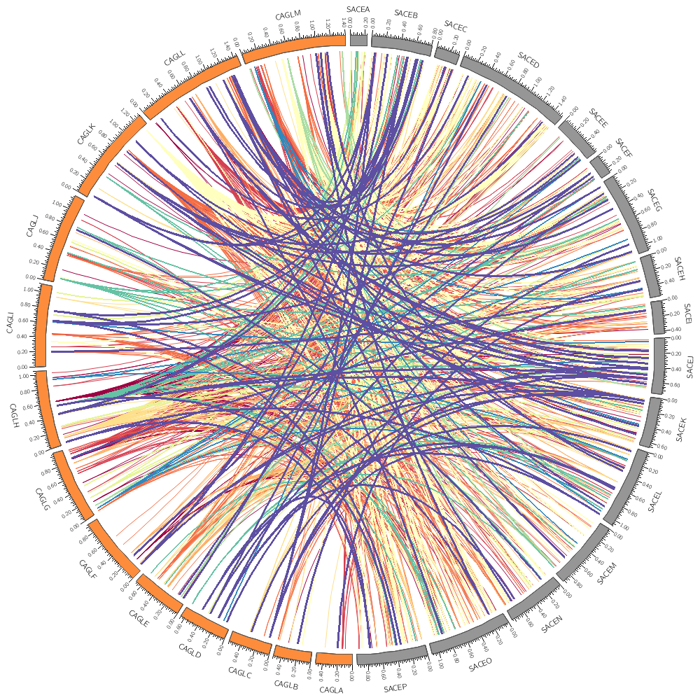
color         = black_a15

Even with _a15 (75% transparency) the image looks quite busy. Try _a20. Now we come to a very powerful part of Circos. Instead of just drawing the data the way it appers in the input file, you can adjust how data points (e.g. histogram bins, links, or anything) can appear based on its properties, such as chromosome, position, size, and so on.

While you can potentially define these parameter in the input files, by applying them to only certain lines in the files that you filtered with a script, it's easier to do it in the configuration file.

Turn the rules on below by setting use=yes.

<rules>
use = yes

One of the simplest ways in which a rule can be used is to turn of the display of data points.

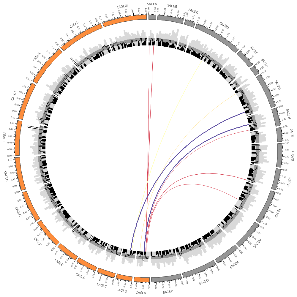
Since our links are regions of conservation, let's only show those that have a size of at least 4 kb. To do this, we set a condition that triggers for links smaller than 4 kb. Any other directives or parameters in the rule will be applied to these links before they're drawn. In this case setting show=no will hide the links.

<rule>
condition     = var(size1) < 4000
show          = no
</rule>

You can change the color of a data point (which may be a point in a scatter plot# bar in a histogram, a link, etc) using any of its other property. Each link here corresponds to a conserved region in CAGL that also appears in SACE and thus the start and end of the link have a size.

The rule below maps the color of the link based on the size of its start given by var(size1) onto the 11-color diverging spectral Brewer palette. Two additional lines change the thickness of the link and its z-depth.

Circos defines a large number of named colors. All these definitions are in the Circos installation directory under etc/. For convenience, I have included these files in colornames/ in this lecture's section.

<rule>
use           = yes

This condition applies to all data points that reach this rule.

condition     = 1

The function remap_int(var,min,max,mapmin,mapmax) linearly maps the value given by var from the range [min,max] to [mapmin,mapmax]. We're using sprintf(fmt,list) to format the value as a string that corresponds to the name of a Brewer color.

The eval() is required to parse the contents as code as opposed to treating them as a string literal.

color         = eval(sprintf("spectral-11-div-%d",remap_int(var(size1),4000,6000,1,11)))
thickness     = eval(sprintf("%d",remap_int(var(size1),4000,6000,1,3)))

Without eval(), z would be set to the literal string "var(size1") and not to the actual value of the size1 parameter.

z             = eval(var(size1))
</rule>
</rules>

</link>
</links>

karyotype = ../../data/karyotype.txt

▲ sessions/day.1/lecture.3/2/circos.png (zoom)

chromosomes_display_default = no
chromosomes = /sace|cagl/

<links>
<link>
file          = ../../data/link_cagl_sace.txt
radius        = 0.80r
bezier_radius = 0r
thickness     = 1
record_limit  = 1000
color         = black_a15

<rules>

<rule>
condition     = var(size1) < 4000
show          = no
</rule>

<rule>
condition     = 1
color         = eval(sprintf("spectral-11-div-%d",remap_int(var(size1),4000,6000,1,11)))
thickness     = eval(sprintf("%d",remap_int(var(size1),4000,6000,1,3)))
z             = eval(var(size1))

</rule>
</rules>

</link>
</links>

Below are the two histograms from the previous lecture. I've used the 50kb binning for both.

Notice that both tracks have the same r0 and r1 values. They are drawn on top of each other. There is no restriction on this.

<plots>
<plot>
file        = ../../lecture.2/5/genes.count.50kb.txt
type        = histogram
fill_color  = vlgrey
stroke_thickness  = 0
r1 = 0.95r
r0 = 0.80r 
orientation = out
</plot>

This histogram has no fill (by default it's not defined) and a black outline.

<plot>
file             = ../../lecture.2/5/genes.avgsize.50kb.txt
type             = histogram
color            = black
stroke_thickness = 1
r1 = 0.95r 
r0 = 0.80r 
orientation = out 

You can reference the min, max, average (avg), standard deviation (sd) of a track using var(plot_STATISTIC). For example, var(plot_avg) gives the average and the rule above, when activated, fills assigns a black fill to bins whose size smaller than track average.

<rules>
use        = no
<rule>
condition  = var(value) < var(plot_avg)
fill_color = black
</rule>
</rules>

<backgrounds>
<background>
color = black_a15
y1 = 2000
y0 = 1500
</background>
</backgrounds>

</plot>

</plots>

karyotype = ../../data/karyotype.txt

▲ sessions/day.1/lecture.3/3/circos.png (zoom)