Learning Circos
Bioinformatics and Genome Analysis
Institut Pasteur Tunis Tunisia, December 10 – December 11, 2018
v2.00 6 Dec 2018 Download PDF slides
v2.00 6 Dec 2018
A 2- or 4-day practical mini-course in Circos, command-line parsing and scripting. This material is part of the Bioinformatics and Genome Analysis course held at the Institut Pasteur Tunis.
Quick links
BCGA 2018 | 1-day Circos course | Circos documentation best practices getting started | Brewer palette swatches | Color resources | Nature Methods Points of View Points of Significance
Getting started with Circos: Yeast and Ebola
Monday 10 December 2018 — Day 1
9h00 - 10h30 | Lecture 1 — Introduction to Circos
11h00 - 12h30 | Lecture (practical) 2 — Visualizing gene distribution and size in Yeast: the histogram data track
14h00 - 15h30 | Lecture (practical) 3 — Conservation in Yeast: the link data track
16h00 - 18h00 | Lecture (practical) 4 — Visualizing an Ebola strain
Concepts covered today
Circos configuration, common Circos errors, Circos debugging, ideograms, selecting ideograms with regular expressions, data tracks, histograms, links, downloading files from UCSC genome browser, essential command-line tools and basic scripting, using bash to create data files for Ebola genome strains, color definitions, using transparency, Brewer palettes, runtime formatting rules, accessing data track statistics, input data formats
Visualizing gene distribution and size in Yeast: the histogram data track
This is our first practical session. It will be a brief introduction to Circos, meant to give you a rough overview. We'll get into more details later.
To get started, let's assume that you have the course materials installed in
DIR=~/circos/course
Switch to this lecture lecture
 cd $DIR
 cd sessions/day.1/lecture.2
 ls
You can save this directory as a shell variable using
>export DIR=~/circos/course
at the terminal or add the line to your .bashrc.
You'll want to explore the numbered directories in this lecture's directory
 1/
 2/
 ...
These are stand-alone parts of the lecture. Anything you do within these directories don't impact other parts of this lecture or other lectures.
cd 1/
Within each part you'll find a configuration directory
etc/
that contains the files used to generate the Circos image. This is the configuration and (at times) data files. In some cases, data files are taken from the day's top directory, such as
day.1/data
To create the image, just execute 'circos' at the prompt within the lecture's part directory
 > pwd
 ~/circos/course/sessions/day.1/leture.2/1
 > circos
 debuggroup summary 0.22s welcome to circos v0.69-7 2 Nov 2017 on Perl 5.010000
 ...
 debuggroup output 7.41s created PNG image ./circos.png (229 kb)
Now look at the output image. You may have to refresh your viewer if you're overwriting the image.
Open the configuration file
etc/circos.conf
in an editor and follow the instructions. Sometimes you'll be asked to make changes and regenerate the image. At other times, you'll need to look at data files and write some scripts.
Central in a Circos figure are the ideograms and their order, scale and orientation.
An ideogram is the graphical depiction of a chromosome and, generally, any stretch of sequence. A chromosome may be shown as a single ideogram, in whole or cropped, or as multiple ideograms, if you divide it into several regions. It is important to create an ideogram layout that helps the reader parse and understand the data.
For example, if you are comparing a single chromosome of one genome (e.g. human chr1) to an entire mammalian genome (e.g. mouse), it is helpful to magnify the human chromosome (e.g. so that it takes 50% of the figure) to present its data at a higher resolution.
On the other hand, if you are comparing two genomes, or roughly equal size subsets of two genomes, it is helpful to scale the ideograms to have the same size to create a pleasing symmetrical layout.
The karyotype defines all our chromosomes (name, label, length, color)
karyotype = ../../data/karyotype.txt
Some system settings that you don't need to worry about right now.
chromosomes_units = 100

<<include ideogram.conf>>
You'll also notice that the ticks and tick labels in this image are very dense. Don't worry about this right now, we'll fix it later.
<<include ../../../etc/ticks.conf>>
<<include ../../../etc/image.conf>>

<<include etc/colors_fonts_patterns.conf>>
<<include etc/housekeeping.conf>>
karyotype = ../../data/karyotype.txt
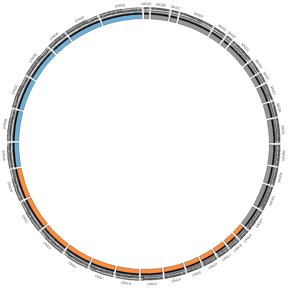
We can draw any subset of chromosomes defined in the karyotype file. This is useful if we have multiple genomes defined (as in this case) and we want to show only one genome.
By default, Circos draws all the chromosomes defined in the karyotype file in the order that they appear. Let's change this by setting the default display.
chromosomes_display_default = no
Now we have to define what chromosome to draw.
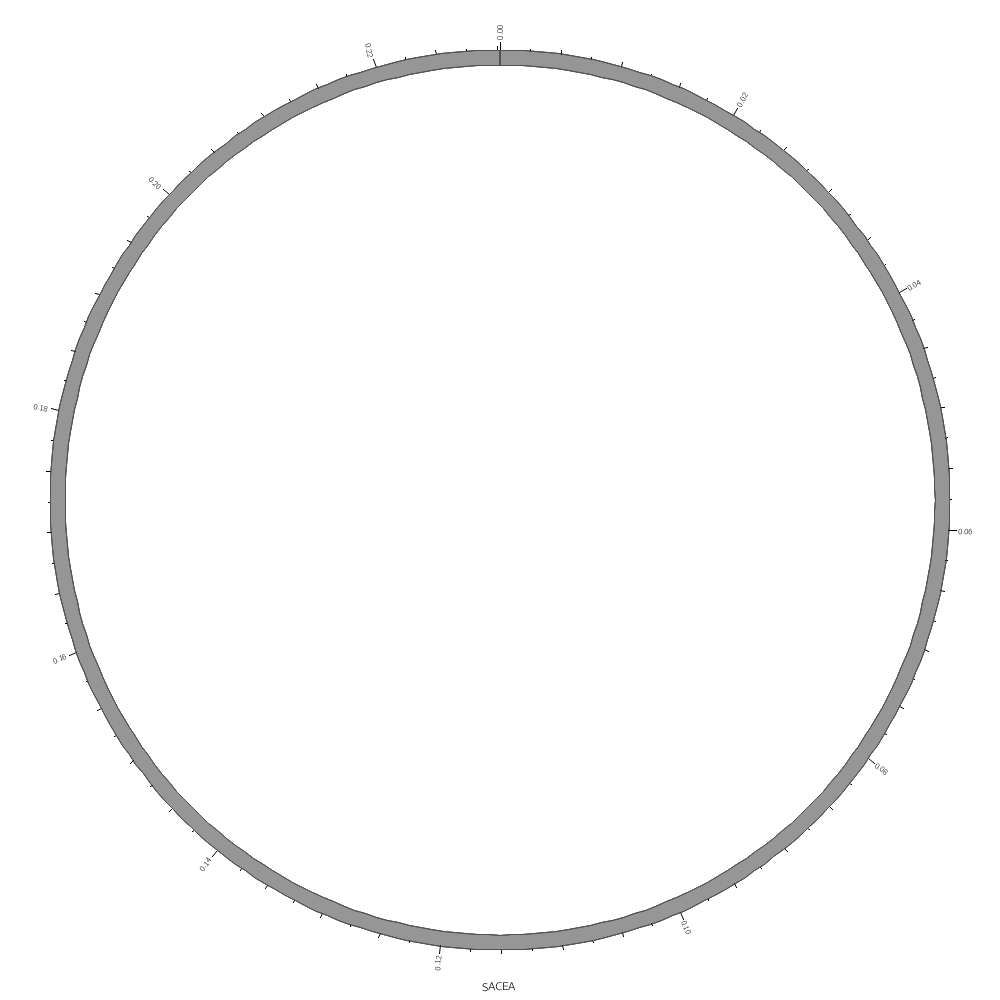
chromosomes = sace-a # draw the sace-a chromosome
If we want to draw more chromosomes from SACE, just add them to the list
#chromosomes = sace-a;sace-b;sace-c;sace-d # a list of chromosomes
But what if we wanted to draw all the SACE chromosomes but didn't really want to have to list them all. For this, use a regular expression.
#chromosomes = /sace/ # regular expression that matches any chromosome with sace substring
There are 36 chromosomes in the karotype file
sace-a ... sace-p
cagl-a ... cagl-m
zyro-a ... zyro-g
Regular expressions are very powerful in matching strings
#chromosomes                = /-a/     # all -a chromosomes
#chromosomes                = /-[abc]/ # all -a, -b or -c chromosomes
karyotype = ../../data/karyotype.txt

chromosomes_display_default = no
chromosomes                 = /sace/
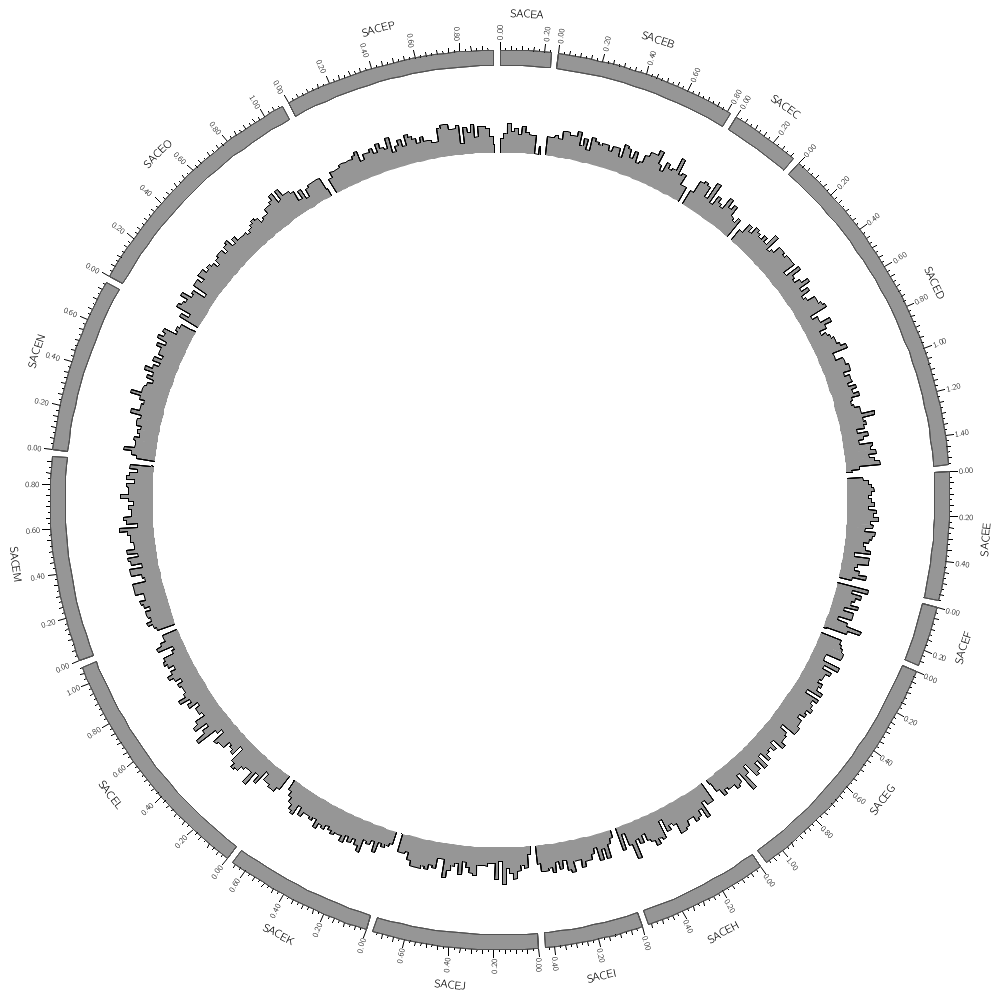
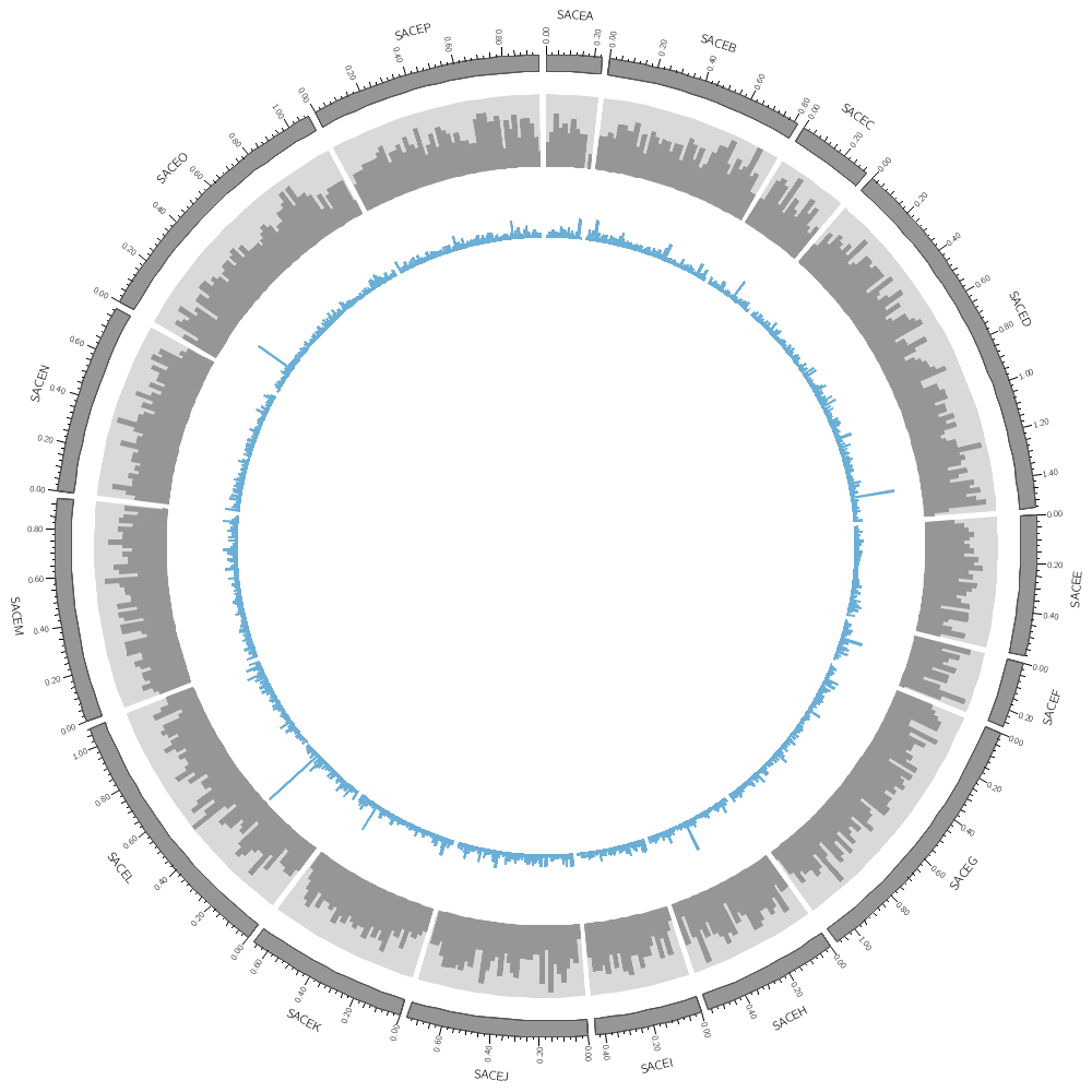
Data tracks are defined in <plot> blocks inside an outer <plots> block Let's plot the gene count for SACE.
<plots>
<plot>
file       = ../../data/genes.count.20kb.txt
type       = histogram
fill_color = grey
stroke_thickness = 1
color     = black
The location of the track is defined by r0 (inner radius) and r1 (outer radius). They are best expressed as a relative fraction of the ideogram radius.
#r0 = 0.7r # track starts at 70% of ideogram radius
#r1 = 0.9r # track ends at 90% of ideogram radius
By default the histogram plot points outward but you can flip it with orientation
#orientation = in # in,out
By default the histogram stroke is placed only on the outside. To add a stroke to each individual bin use stroke_type
#stroke_type = both # both,outline

</plot>  # don't forget the closing tag
Now let's add another plot. We'll also plot the average gene size. Notice that use=no in this plot — this turns the plot off. To turn it on, set it to yes
<plot>
use              = no # no,yes
file             = ../../data/genes.avgsize.10kb.txt
type             = histogram
fill_color       = blue
stroke_thickness = 0

r0 = 0.7r
r1 = 0.5r

orientation = out

</plot>

</plots>
karyotype = ../../data/karyotype.txt

chromosomes_display_default = no
chromosomes                 = /sace/

<plots>
<plot>
file        = ../../data/genes.count.20kb.txt
type        = histogram
fill_color  = grey
stroke_thickness  = 0
r1 = 0.95r
r0 = 0.80r
orientation = out
Backgrounds are defined in their own blocks. If you have a single <background> block then by default the background will fill the track.
<backgrounds>
<background>
color = vlgrey
</background>
Multiple backgrounds are layered. This one is turned off (use=no) so turn it back on.
<background>
use   = no
color = lorange
y0    = 0.75r   # starts at 75% from bottom of plot
</background>
</backgrounds>
</plot>

<plot>
file             = ../../data/genes.avgsize.10kb.txt
type             = histogram
fill_color       = blue
stroke_thickness = 0
r1 = 0.79r
r0 = 0.65r
orientation = out
<backgrounds>
use   = no     # use is inherited by all children blocks
<background>
color = vlblue
</background>
<background>
color = lblue
y1    = 5000   # absolute value of end of background
y0    = 2500   # absolute value of start of background
</background>
</backgrounds>

</plot>

</plots>
karyotype = ../../data/karyotype.txt
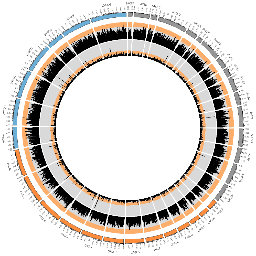
Let's draw all three genomes: SACE, CAGL and ZYRO
chromosomes_display_default = yes
Our data was binned into 20 kb bins for the gene count and 10 kb bins for gene average size. You'll notice that when you run Circos, it tells you that the total size of all chromosomes is 34 Mb.
...
karyotype has 36 chromosomes of total size 34,154,242
...
This means that we have about 3,400 bins for the gene size histogram and 1,700 bins for the gene count histogram. Because we have so many bins, they're thin and hard to see.
We'll need to resample the data into bigger bins. For this, see the resample.sh script in this directory, which uses one of the helper tools of Circos.
Once you've created the new files, change the file parameter in the <plot> blocks to point to the new files. Note that the files are in the current directory, so you don't need ../../
Which bin size looks best for you?
Once you've run the log transforms, plot those data too. Do any of the tracks benefit from this transform? Note that for the size track, you'll need to change the background y0 and y1 values to their corresponding log transformed values
To learn about visual acuity and guidelines for controlling the size of elements on the screen or page, see
handout/visual.acuity.points.pdf
For background reading about managing resolution for print, see
handout/figure.size.resolution.pdf
I will have a printed copy of both of these handouts — it is important that you see what different size elements and type look like on paper.
<plots>
<plot>
Once you've generated rebinned data, change the file here.
file        = ../../data/genes.count.20kb.txt
type        = histogram
fill_color  = black
stroke_thickness  = 0
r1 = 0.95r
r0 = 0.80r
orientation = out

<backgrounds>
<background>
color = vlgrey
</background>
<background>
color = lorange
y0    = 0.75r
</background>
</backgrounds>
</plot>

<plot>
file             = ../../data/genes.avgsize.10kb.txt
type             = histogram
fill_color       = black
stroke_thickness = 0
r1 = 0.79r
r0 = 0.65r
orientation = out
<backgrounds>
<background>
color = vlgrey
</background>
<background>
color = lorange
y1    = 5000
y0    = 2500
</background>
</backgrounds>

</plot>

</plots>
#!/bin/bash

# This is the directory where the Circos tools are installed
# on my computer at work. But for your setup, it'll be different.
# Change this to the right directory. Take a look in /root/modules/circos
# to find it.
CTOOLS=/home/martink/work/circos/svn/tools/

# Let's make data sets for both the count and average size for 50, 75 and 100 kb

for binkb in 50 75 100 ; do

  binsize=$((1000*binkb))

  echo "Resampling at $binsize"
  cat ../../data/genes.txt | $CTOOLS/resample/bin/resample -bin $binsize -count > genes.count.${binkb}kb.txt
  cat ../../data/genes.txt | $CTOOLS/resample/bin/resample -bin $binsize -avg   > genes.avgsize.${binkb}kb.txt

done

# Look at the manpage of the 'resample' script by running 'resample -man' You'll notice
# that it can also report the minimum and maximum values in a bin. Add these
# to the loop above to create files for these variables (e.g. genes.maxsize.100kb.txt)
#
# You transform the vertical scale in Circos but you can also do it
# when generating the data file. Here 'awk' is very helpful and its log() function
# which gives the natural logarithm. So log(x)/log(10) is the base 10 logarithm.

cat genes.count.50kb.txt | awk '{print $1,$2,$3,log($4)/log(10)}' > genes.count.50kb.log.txt

# Write a loop that applies this transformation to all the bins (50, 75, 100 kb) and all the
# quantities (count, avg, min, max). Watch out for bins with value 0 — the log() call
# will produce an error. How would you deal with this?