

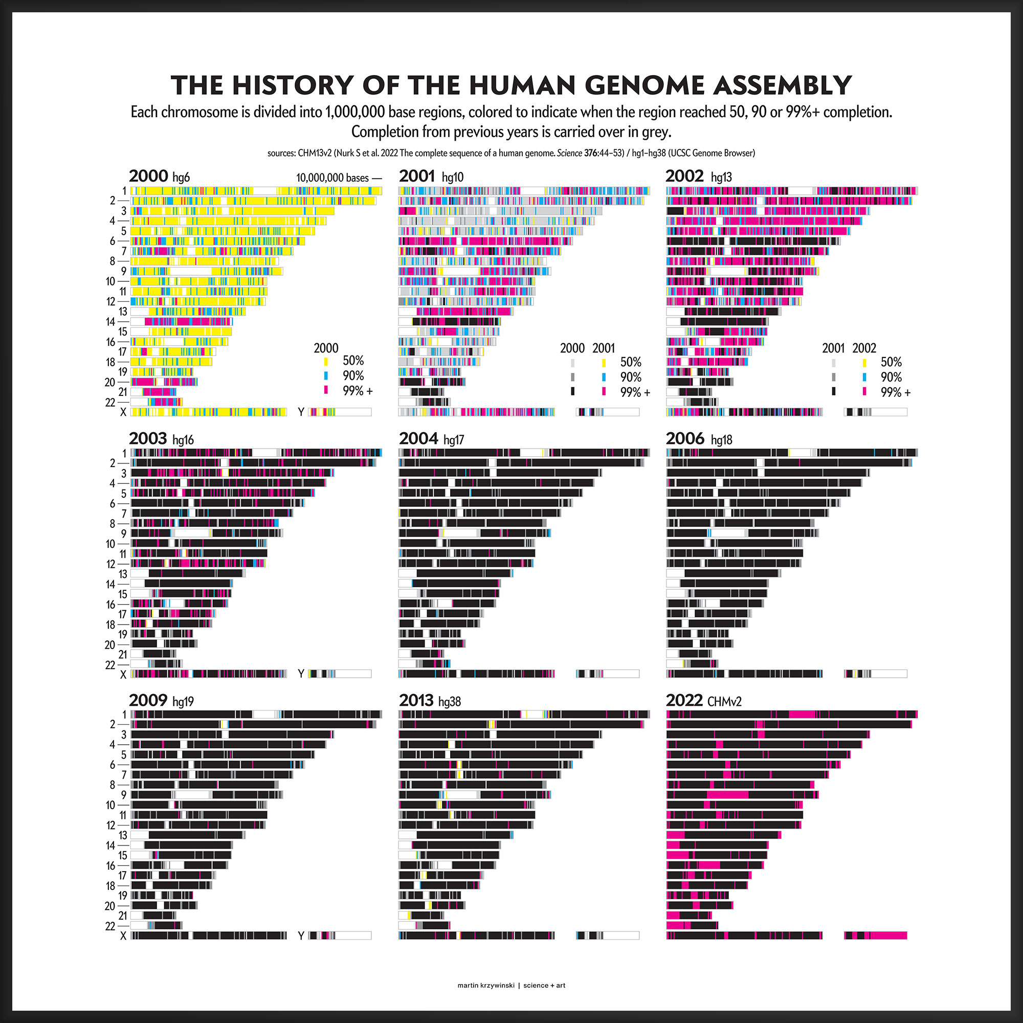
History of the Human Genome Assembly
22 years, 3,117,275,501 bases and 0 gaps later
Round numbers are always false.
— Samuel Johnson
Here, you can expect to learn about the history of the human genome assembly (and a little bit about its structure) and see a map of its completion over the last 22 years, which was published in Scientific American Graphic Science.
contents
In March 2022, a flurry of publications announced the first ever complete assembly of a human genome. This is a big deal because, in genomics, we don't throw around words like “complete” very often. Actually, never — until now.
Because the human genome — a human genome — is complete. All hail the CHM13v2 (Mar 2022) telomere-to-telomere (T2T) assembly.
You've probably already heard — and have been hearing for the last 15 years — that the human genome has been sequenced. After all, how else can there be a publication with the title Finishing the euchromatic sequence of the human genome (2004 Nature 431:931–945).
In 2004, the only thing that stood between “finished” and “complete” was that pesky word “euchromatic”.
“Euchromatin is a lightly packed form of chromatin (DNA, RNA, and protein) that is enriched in genes, and is often (but not always) under active transcription. Euchromatin stands in contrast to heterochromatin, which is tightly packed and less accessible for transcription. 92% of the human genome is euchromatic.” — Wikipedia
For modeling and analysis — such as in cancer research, for example, which is what we do here — by far the most important parts of the human genome assembly are the parts that code for protein (transcribed regions and their ORFs), along with their adjacent regulatory sequences.
These regions in total occupy less than half of the genome. The parts that ultimately translated into protein exons account for just 2.58% of the genome. For the vast majority of genes, the sequence in these regions was indeed finished.
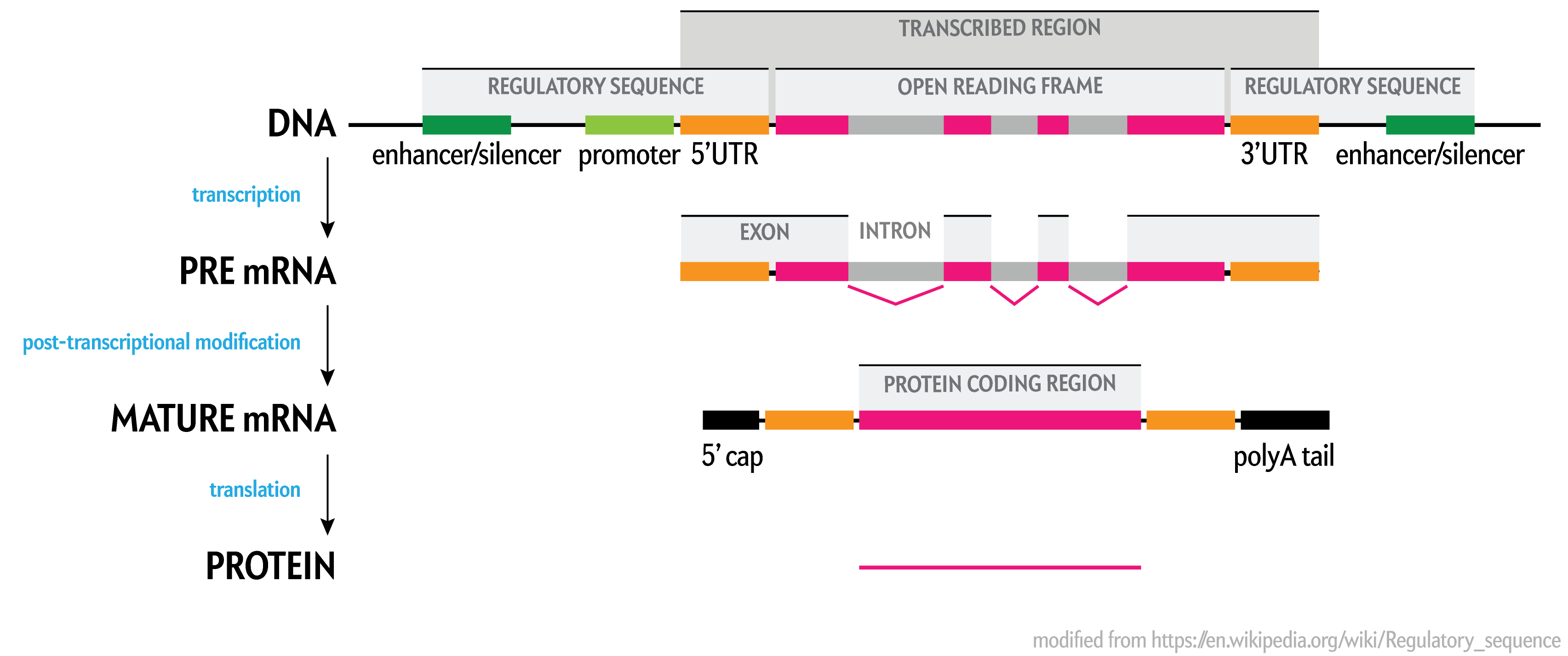
In the most recent assembly prior to the complete telomere-to-telomere CHM13v2 assembly was hg38 (Dec 2013), exons cover only 2.58% of the total sequence (excluding gaps) of the assembly. Notice how much of the open reading frame (ORF) is in introns, which are spliced out during post-transcriptional modification into mature mRNA.
The values in the table above are generated from the size of the union of assembly intervals over the set of genes, because some genes overlap The list of genes includes protein coding, non-coding and pseudogenes.
But with the CHMv2 assembly being more than 200 million bases larger (hello heterochromatin!), we expect to find more genes. And indeed, 3,604 genes, of which 140 are protein coding, are exclusive to CHMv2 (Table 1 in Nurk et al.).
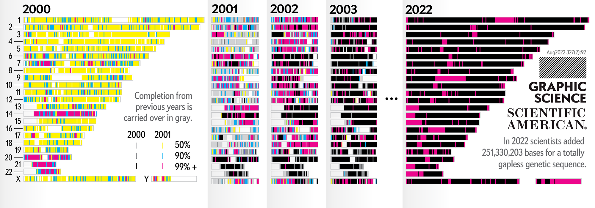
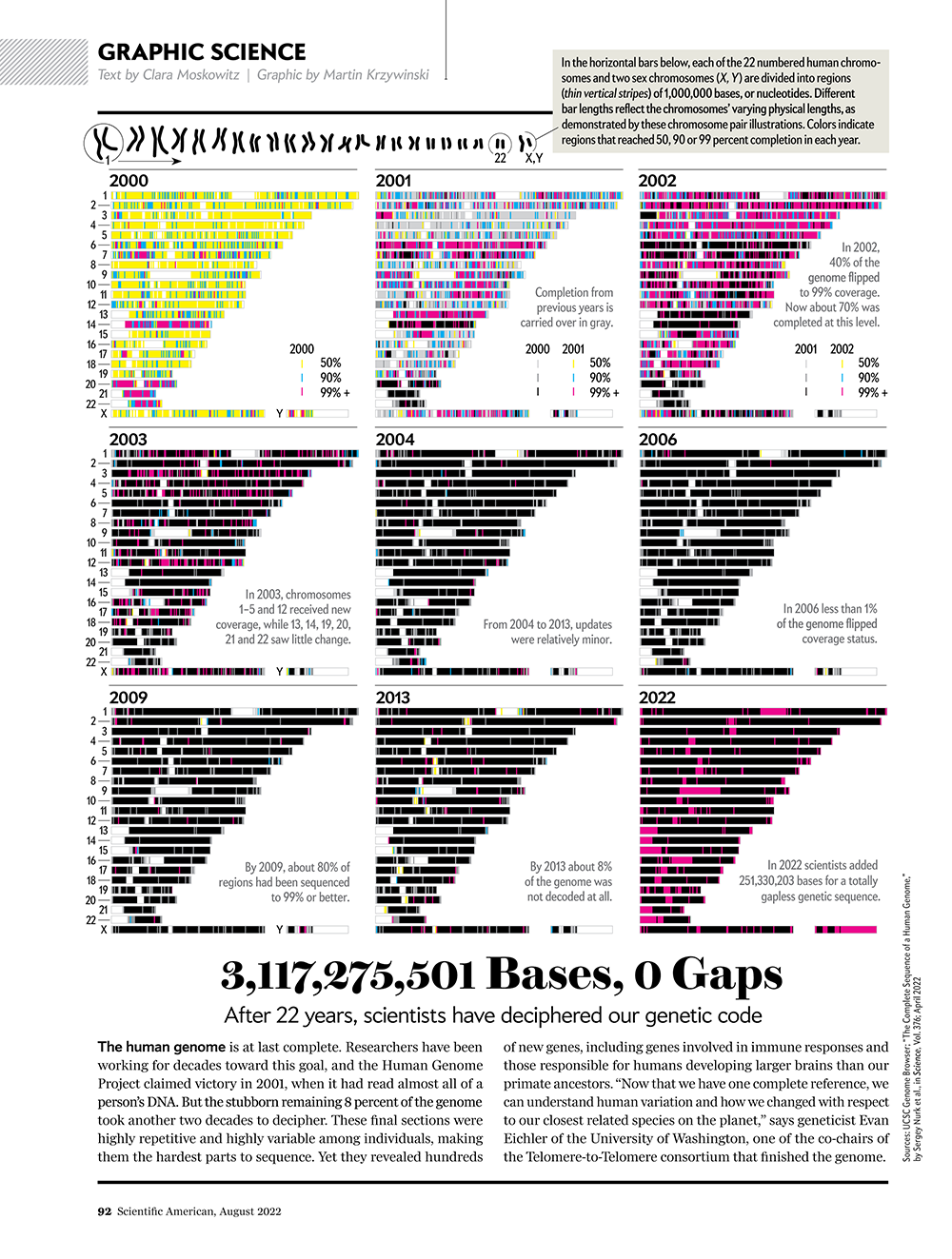
Our goal for the August 2022 Scientific American Graphic Science page was to present the CHMv2 assembly in context of the efforts of the past 22 years — as the final sequencing stage in the sequencing effort. See my other Graphic Science illustrations.
 buy artwork
The DNA samples used to create the reference human sequence assembly used DNA samples from multiple individuals.
The bulk of the genome was sequenced from the RPCI-11 genomic library, which is a collection of about 10,000 randomly sampled pieces (each on average 180,000 bases long) from the genome of an individual male. Other parts of the genome assembly were reconstructed by sequencing RPCI-13 (female) and Caltech-D (Table 2 in Zhao (2000)) libraries.
The human genome is a variable quantity — two individuals vary, on average, by 1 base in 1,000 (or, roughly, in about 3 million positions) — and much of human genomics deals with understanding and handling this variability.
As such, the term “the human genome” is a little misleading and it's important to acknowledge that, given this natural variation between individuals (and even between cells within an individual), there is really no such thing.
When we say “the genome” we invariably mean “the reference genome”. Even then, we need to specify which version of the reference we mean. At the moment (July 2022), the hg38 (Dec 2013) assembly is considered to be the canonical reference and this may not change anytime soon. It's not uncommon (especially for several months after the release of a new assembly) to find genomic resources that use older references — updating an analysis or data pipeline to a new reference assembly is not a trivial task.
For example, well after the release of hg38 (Dec 2013), the previous reference hg19 (Feb 2009) continued to be widely used for several years. To facilitate standardizing results to the same assembly, so-called liftOver annotations allow conversion of one assembly's coordinates to another.
As the sequence assembly matured, regions were successively filled in by targeted efforts focusing on specific regions (e.g. DNA sequence analysis of human chromosome 9) or by specific institutions (e.g. A Japanese history of the Human Genome Project).
This kind of focused effort to improve the assembly quality of a region was always part of the process. In fact, already in 2000 you can see that significant portions of chromosomes 14, 20, 21 and 22 were completed to 99%+. In 2001, chromosomes 6 and 13 received a lot of attention.
In contrast to focused sequencing, other parts of the assembly were sequenced in a shotgun fashion — by randomly sampling as many regions in the genome as possible in an effort to spread out the coverage. Early on, the shotgun effort was accelerated so that the public assembly would provide more coverage (with commensurately higher quality) than the private sector assembly created by Celera.
Over the years 2000 to 2013, the human genome assembly progressively improved from a so-called “draft” assembly to one that, practically, may be called “finished” (finishish?). These terms can be defined in various ways — for example, based on how much of coding sequence is represented, the contiguity of the assembly, the total coverage of the genome, or some combination of these metrics.
Individual assemblies were indexed by hgN from hg1 (May 2000) to hg38 (Dec 2013). Differences in the index value do not necessarily represent how much of the assembly changed and some indexes were skipped. And I'm still trying to locate the sequence files of hg3 (July 2000).
The hg prefix was used by the team at the UCSC Genome Browser while NCBI had their own assembly build indexes (e.g. hg10 was NCBI build 28). In fact, as of July 2022, there are 1,268 assemblies of the human genome indexed by NCBI.
The hg38 (Dec 2013) assembly continues to be the canonical “reference sequence” since 2013 (and likely beyond 2022). An excellent assembly, it nevertheless contains 1,001 gaps totalling about 150 Mb across chromosomes 1–22, X and Y. as well as 430 unanchored and alternate pieces that totalled 121 Mb and themselves include 240 gaps of about 9 Mb.
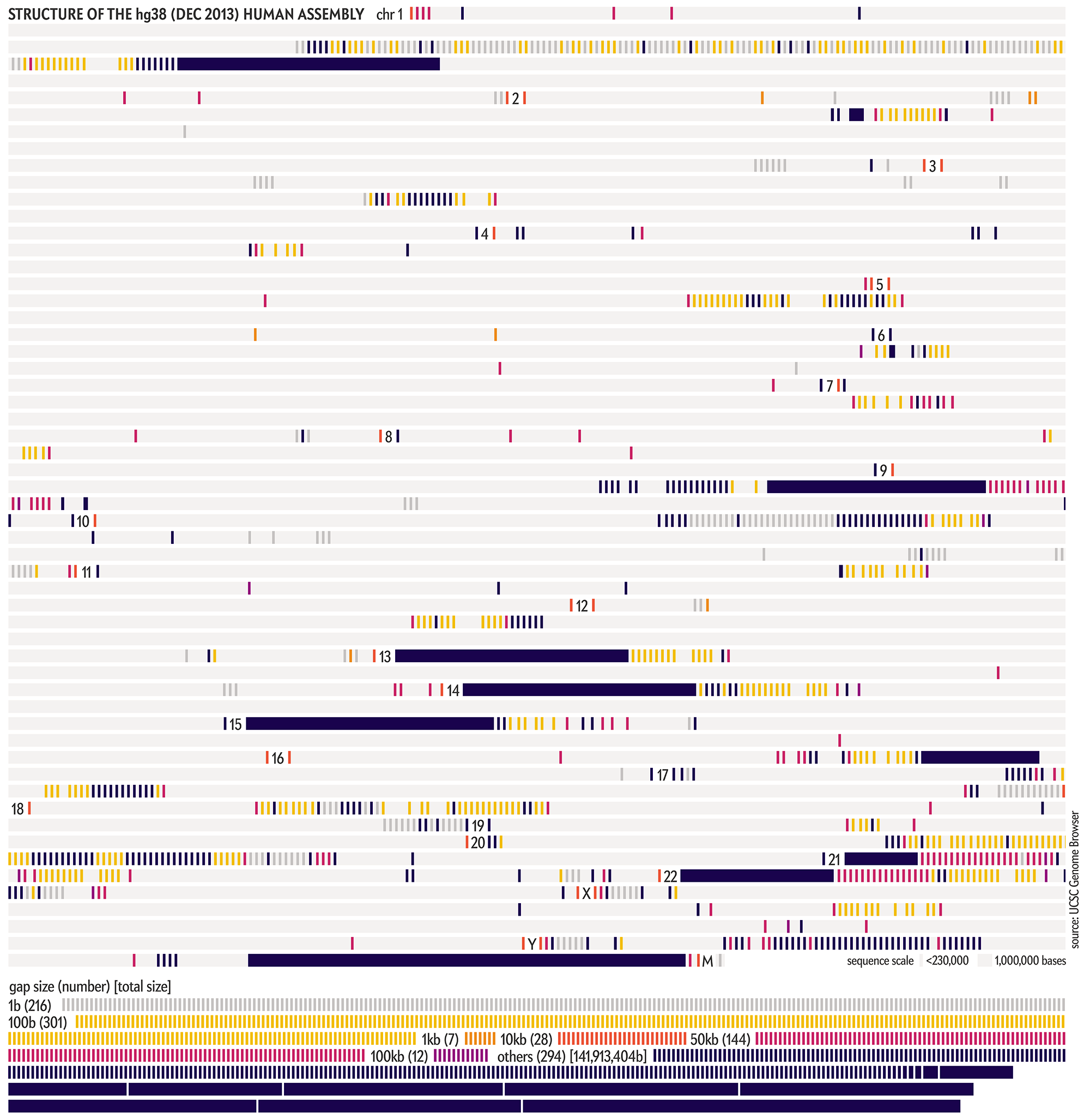
These gaps were mostly in heterochromatic regions, which are notoriously difficult to sequence. When the size of the gap was not known, following tradition, it was set to 100 bases . Other sizes, such as 1kb, 10kb and 50kb signalled more information about the nature of the gap, such as a contig gap, short arm gap, telomere gap, and so on.
The CHM13v2 (Mar 2022) assembly filled in all these gaps. It is a completely gapless assembly.
Nasa to send our human genome discs to the Moon
We'd like to say a ‘cosmic hello’: mathematics, culture, palaeontology, art and science, and ... human genomes.


Comparing classifier performance with baselines
All animals are equal, but some animals are more equal than others. —George Orwell
This month, we will illustrate the importance of establishing a baseline performance level.
Baselines are typically generated independently for each dataset using very simple models. Their role is to set the minimum level of acceptable performance and help with comparing relative improvements in performance of other models.

Unfortunately, baselines are often overlooked and, in the presence of a class imbalance5, must be established with care.
Megahed, F.M, Chen, Y-J., Jones-Farmer, A., Rigdon, S.E., Krzywinski, M. & Altman, N. (2024) Points of significance: Comparing classifier performance with baselines. Nat. Methods 20.
Happy 2024 π Day—
sunflowers ho!
Celebrate π Day (March 14th) and dig into the digit garden. Let's grow something.

How Analyzing Cosmic Nothing Might Explain Everything
Huge empty areas of the universe called voids could help solve the greatest mysteries in the cosmos.
My graphic accompanying How Analyzing Cosmic Nothing Might Explain Everything in the January 2024 issue of Scientific American depicts the entire Universe in a two-page spread — full of nothing.

The graphic uses the latest data from SDSS 12 and is an update to my Superclusters and Voids poster.
Michael Lemonick (editor) explains on the graphic:
“Regions of relatively empty space called cosmic voids are everywhere in the universe, and scientists believe studying their size, shape and spread across the cosmos could help them understand dark matter, dark energy and other big mysteries.
To use voids in this way, astronomers must map these regions in detail—a project that is just beginning.
Shown here are voids discovered by the Sloan Digital Sky Survey (SDSS), along with a selection of 16 previously named voids. Scientists expect voids to be evenly distributed throughout space—the lack of voids in some regions on the globe simply reflects SDSS’s sky coverage.”
voids
Sofia Contarini, Alice Pisani, Nico Hamaus, Federico Marulli Lauro Moscardini & Marco Baldi (2023) Cosmological Constraints from the BOSS DR12 Void Size Function Astrophysical Journal 953:46.
Nico Hamaus, Alice Pisani, Jin-Ah Choi, Guilhem Lavaux, Benjamin D. Wandelt & Jochen Weller (2020) Journal of Cosmology and Astroparticle Physics 2020:023.
Sloan Digital Sky Survey Data Release 12
Alan MacRobert (Sky & Telescope), Paulina Rowicka/Martin Krzywinski (revisions & Microscopium)
Hoffleit & Warren Jr. (1991) The Bright Star Catalog, 5th Revised Edition (Preliminary Version).
H0 = 67.4 km/(Mpc·s), Ωm = 0.315, Ωv = 0.685. Planck collaboration Planck 2018 results. VI. Cosmological parameters (2018).
constellation figures
stars
cosmology
Error in predictor variables
It is the mark of an educated mind to rest satisfied with the degree of precision that the nature of the subject admits and not to seek exactness where only an approximation is possible. —Aristotle
In regression, the predictors are (typically) assumed to have known values that are measured without error.
Practically, however, predictors are often measured with error. This has a profound (but predictable) effect on the estimates of relationships among variables – the so-called “error in variables” problem.

Error in measuring the predictors is often ignored. In this column, we discuss when ignoring this error is harmless and when it can lead to large bias that can leads us to miss important effects.
Altman, N. & Krzywinski, M. (2024) Points of significance: Error in predictor variables. Nat. Methods 20.
Background reading
Altman, N. & Krzywinski, M. (2015) Points of significance: Simple linear regression. Nat. Methods 12:999–1000.
Lever, J., Krzywinski, M. & Altman, N. (2016) Points of significance: Logistic regression. Nat. Methods 13:541–542 (2016).
Das, K., Krzywinski, M. & Altman, N. (2019) Points of significance: Quantile regression. Nat. Methods 16:451–452.