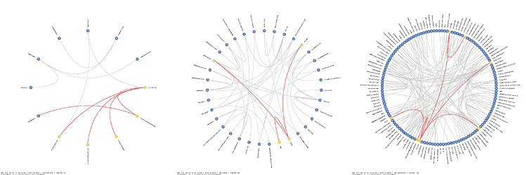
Schemaball
Circular visualization of database schemas
Schemaball was published in SysAdmin Magazine (Krzywinski, M. Schemaball: A New Spin on Database Visualization (2004) Sysadmin Magazine Vol 13 Issue 08). Who cites Schemaball?
These tutorials illustrate different features of Schemaball. Tutorials are divided into sections. Each section covers a particular aspect of a feature or set of features. Each section has its own documentation, configuration file and schema ball image.
tutorial 2
Extracting and drawing constraint relationships.
NAME
sbtut_02 - extracting and drawing constraint relationships
SYNOPSIS
  <linkrule fieldregex>
  fieldrx   = ^(\w+)_([a-z]+)$
  use       = yes
  avoidself = yes
  <fields>
  table = 0
  field = 1
  </fields>
  </linkrule>
  <link>
  show_links = yes
  color  = cccccc
  stroke = 2
  anchor = edge
  type = bezier
  </link>
  <bezier>
  resolution = 100
  radius = 0.1
  </bezier>
PURPOSE
Schemaball can parse constraint relationships in a number of ways. It understands ``CONSTRAINT'' table options, it can parse field names to generate constraints and read constraints from external flat files. In this tutorial, we'll use the Ensembl human genome database to show how foreign key status can be parsed from field names.
TUTORIAL
MySQL does not supports foreign keys for MyISAM tables as of version 4.0. Consequently, application logic is required to maintain constraints and database integrity. To aid in this process, developers name foreign key fields in a distinct manner, so that these fields may be easily recognized.
Parsing Constraints
In the Ensembl schema, foreign keys are named with the convention TABLENAME_FIELD, where TABLENAME is the name of the target table and FIELD is the field name.
To instruct Schemaball how to parse constraints from field names, a <linkrule> block is used with a 'fieldrx' parameter. This parameter defines the regular expression applied to the field name. Cpture brackets delineate the target table and target field and the ordinality of these brackets is stored in the <fields> subblock.
For example, the table density_type contains these fields:
  density_type_id int(11) NOT NULL auto_increment,
  analysis_id int(11) NOT NULL default '0',
  block_size int(11) NOT NULL default '0',
  value_type enum('sum','ratio') NOT NULL default 'sum',
The analysis_id is a foreign key which points to the table analysis and the field analysis_id. The regular expression to parse this naming convention is therefore ``^([a-z_]+)_([a-z])+$''. The first capture bracket, which defines the target table, includes a ``_'' in the character class because tables may contain this character. Schemaball will perform a sanity check to make sure that the target field exists within the target table. In this specific case, since analysis.id does not exist, a check for analysis.analysis_id will be made.
The appropriate <linkrule> block, which is a named block and may be given an arbitrary name, is <linkrule fieldregex> fieldrx = ^(\w+)_([a-z]+)$ use = yes avoidself = yes <fields> table = 0 field = 1 </fields> </linkrule>
The 'avoidself' parameter removes any foreign keys which appear to be self-referencing.
Configuration
In addition to the <linkrule> block, a <link> subblock is used to format the constraint lines.
  <link>
  show_links = yes
  color  = cccccc
  stroke = 2
  anchor = edge
  type = bezier
  </link>
The 'anchor' determines whether the line will joint the table glyph at its edge, closest to the center of the circle, or at its center. The 'type' determines whether the constraint line is a straight 'line' or a 'bezier' curve. If 'bezier' is used, a <bezier> block is required to define the third point, as well as the rate at which the bezier curve is sampled. The third point is always placed so that its angular component bisects the angle formed by the start and end of the curve. The radial component is specified by 'radius', relative to the radius of the circle.
  <bezier>
  resolution = 100
  radius = 0.1
  </bezier>
Parsing the Schema
To parse the schema and produce the schema diagram,
> schemaball -conf tutorial/02/sbtut_022.conf -debug > parsed.txt
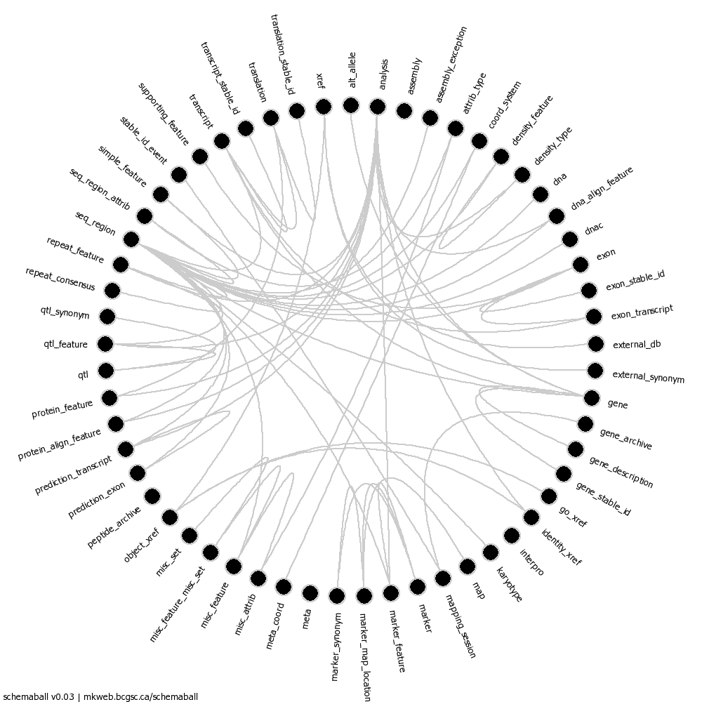
The diagram is included as sbtut_02.png.
Schemaball generates useful information about the schema when the -debug flag is used.
- schema dump
Now that the constraint relationships can be extracted from the schema, the ``schemadump'' lines in Schemaball's output contain these constraints.
  > grep schemadump parsed.txt
  ...
  debug schemadump table coord_system
  debug schemadump table density_feature
  debug schemadump constraint density_feature density_type
  debug schemadump constraint density_feature seq_region
  debug schemadump table density_type
  debug schemadump constraint density_type analysis
  ...
The constraint lines list the source table first, and then the target table.
HISTORY
BUGS
Please report errors and suggestions to martink@bcgsc.ca
AUTHOR
Martin Krzywinski, mkweb.bcgsc.ca, martink@bcgsc.ca
$Id: schemaball,v 1.5 2003/10/27 20:25:11 martink Exp $
CONTACT
  Martin Krzywinski
  Genome Sciences Centre
  Vancouver BC Canada
  www.bcgsc.ca
  mkweb.bcgsc.ca
  martink@bcgsc.ca
configuration
################################################################
#
# Schemaball configuration file
#
# Tutorial 02
#
# sbtut_02_01.conf - fetching and parsing SQL schemas with the Ensembl homo sapiens database
#

<db>
sqlfile = tutorial/02/hs.sql
</db>

<linkrule fieldregex>
fieldrx   = ^(\w+)_([a-z]+)$
use       = yes
avoidself = yes
<fields>
table = 0
field = 1
</fields>
</linkrule>

<image>

file        = /home/httpd/htdocs/worldatwar/schema.png
size        = 1000
glyphradius = 0.7

image_element_dump = yes

background  = ffffff
foreground  = 000000

<elements>

<link>
show_links = yes
color  = cccccc
stroke = 2
anchor = edge
type = bezier
</link>

<bezier>
resolution = 100
radius = 0.1
</bezier>

<label>
font   = tahoma.ttf
size   = 10
</label>

<table>
size    = 25
fill    = 000000
stroke  = 2
outline = cccccc
</table>

</elements>

</image>
Nasa to send our human genome discs to the Moon
We'd like to say a ‘cosmic hello’: mathematics, culture, palaeontology, art and science, and ... human genomes.


Comparing classifier performance with baselines
All animals are equal, but some animals are more equal than others. —George Orwell
This month, we will illustrate the importance of establishing a baseline performance level.
Baselines are typically generated independently for each dataset using very simple models. Their role is to set the minimum level of acceptable performance and help with comparing relative improvements in performance of other models.

Unfortunately, baselines are often overlooked and, in the presence of a class imbalance5, must be established with care.
Megahed, F.M, Chen, Y-J., Jones-Farmer, A., Rigdon, S.E., Krzywinski, M. & Altman, N. (2024) Points of significance: Comparing classifier performance with baselines. Nat. Methods 20.
Happy 2024 π Day—
sunflowers ho!
Celebrate π Day (March 14th) and dig into the digit garden. Let's grow something.

How Analyzing Cosmic Nothing Might Explain Everything
Huge empty areas of the universe called voids could help solve the greatest mysteries in the cosmos.
My graphic accompanying How Analyzing Cosmic Nothing Might Explain Everything in the January 2024 issue of Scientific American depicts the entire Universe in a two-page spread — full of nothing.

The graphic uses the latest data from SDSS 12 and is an update to my Superclusters and Voids poster.
Michael Lemonick (editor) explains on the graphic:
“Regions of relatively empty space called cosmic voids are everywhere in the universe, and scientists believe studying their size, shape and spread across the cosmos could help them understand dark matter, dark energy and other big mysteries.
To use voids in this way, astronomers must map these regions in detail—a project that is just beginning.
Shown here are voids discovered by the Sloan Digital Sky Survey (SDSS), along with a selection of 16 previously named voids. Scientists expect voids to be evenly distributed throughout space—the lack of voids in some regions on the globe simply reflects SDSS’s sky coverage.”
voids
Sofia Contarini, Alice Pisani, Nico Hamaus, Federico Marulli Lauro Moscardini & Marco Baldi (2023) Cosmological Constraints from the BOSS DR12 Void Size Function Astrophysical Journal 953:46.
Nico Hamaus, Alice Pisani, Jin-Ah Choi, Guilhem Lavaux, Benjamin D. Wandelt & Jochen Weller (2020) Journal of Cosmology and Astroparticle Physics 2020:023.
Sloan Digital Sky Survey Data Release 12
Alan MacRobert (Sky & Telescope), Paulina Rowicka/Martin Krzywinski (revisions & Microscopium)
Hoffleit & Warren Jr. (1991) The Bright Star Catalog, 5th Revised Edition (Preliminary Version).
H0 = 67.4 km/(Mpc·s), Ωm = 0.315, Ωv = 0.685. Planck collaboration Planck 2018 results. VI. Cosmological parameters (2018).
constellation figures
stars
cosmology
Error in predictor variables
It is the mark of an educated mind to rest satisfied with the degree of precision that the nature of the subject admits and not to seek exactness where only an approximation is possible. —Aristotle
In regression, the predictors are (typically) assumed to have known values that are measured without error.
Practically, however, predictors are often measured with error. This has a profound (but predictable) effect on the estimates of relationships among variables – the so-called “error in variables” problem.

Error in measuring the predictors is often ignored. In this column, we discuss when ignoring this error is harmless and when it can lead to large bias that can leads us to miss important effects.
Altman, N. & Krzywinski, M. (2024) Points of significance: Error in predictor variables. Nat. Methods 20.
Background reading
Altman, N. & Krzywinski, M. (2015) Points of significance: Simple linear regression. Nat. Methods 12:999–1000.
Lever, J., Krzywinski, M. & Altman, N. (2016) Points of significance: Logistic regression. Nat. Methods 13:541–542 (2016).
Das, K., Krzywinski, M. & Altman, N. (2019) Points of significance: Quantile regression. Nat. Methods 16:451–452.