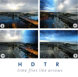
HDTR | High Dynamic Time Range Images
capturing the flow of time in a single frame
contents
- what is HDTR?
- compositing time strips
- temporal blending
- HDTR images of Burrard Bridge
- direction of time flow
- extending the golden hour
- spatial blending
gallery
Browse my HDTR gallery
links
In this section, I describe how I make HDTR images. A lot of this is not going to be useful to you, unless you are implementing your own HDTR application. The majority of readers will be well served by reading the introduction and then browsing the gallery. If you want to take a stab at making your own HDTRs, take a look at the tutorial. All you need are a few images and an image manipulation program.
In this section I address some of the basic questions that arise when attempting to make HDTR images and a few solutions that I've come up with to address basic problems.
- what are the best images?
- how can images be collected?
- what is the (my) approach to blending images
- how to limit banding artefacts
- how to increase contribution from some input images
suitability and collection of images
To make an HDTR image you need at least two images, taken some time apart. There are no rules, so go with what you think will look best. There are a few things to keep in mind though.
First, depending on how quickly your scene is changing (light, traffic, weather patterns), you will need to sample the scene accordingly. Many of the HDTR images in the gallery were created from input images taken every 5 minutes. This is a reasonable periodicity. In some cases, when the light is changing rapidly, images may be taken as frequently as every 1-2 minutes. The effect changing image capture rate is an increase in the contribution of some images towards the final HDTR composite.
In the tutorial, I show how to construct an HDTR images from four input images with Photoshop. As you can see, the result is reasonable without having to take a lot of images. You can imagine doing this from a view from your home or a tripod setup at sunset during a hike, for example.
The images you collect to make an HDTR composite need to fulfill some basic requirements, to lessen the effort required on your part. If you are using a film camera, make sure that you have the aperture set to manual. If you have a digital camera, not only set the camera on manual but also make sure that white blance is not set to auto. Set it to daylight, or something appropriate. Better yet, shoot RAW if you can and put a grey card in your frame, someone off in the corner. If you're using film, then white blance is not an issue, unless you're switching film.
Automatically shifting white balance causes images to have a colour tint (see this set of katkam images for an example of how auto white balance can introduce a tint), which may come and go between time-adjacent frames. Removing this tint is possible but tedious. If you're using a web cam which only supports auto white balance, don't worry about it too much.
One of the artefacts that show up in HDTR images are bands along the input image boundary lines. This is expected since between one image and the next the lighting may have shifted, resulting in a darker/brighter image. Two ways of dealing with this are spatial and temporal blending, discussed below. However, you should do whatever you can to mitigate this issue by collecting well exposed images. In general, since you want to depict the changing scene in your HDTR composite, I suggest a fixed exposure throughout your collection process. If it's a sun day, pick f/16 1/ISO shutter speed, for example. If you're collecting images over an entire day, which includes dawk and dusk, you will need to adjust the exposure to prevent the darker frames from blocking up. When doing this, ramp the exposure slowly (e.g. 1/3 f-stop if your camera supports it, or at most 1/2 f-stop) at the start and end of the day.
If you're on the Canon platform, consider investing in a TC-80N3 remote. It may seem pricey at first, but it's a boon for extended exposure and time lapse photography.
For example, this set of extended exposure photos (bottom of set) was taken using the TC-80N3. I set the camera to take 2 minute exposures continuously and walked away. The TC-80N3 is terrific for campfires, too. In this image, I used a rear-curtain flash after a 30s exposure. I took lots of images like this during the camp fire and didn't have to attend to the camera at all. In some frames, subject movement made the images unuseable. A few were keepers, though. Without the TC-80N3 I could not have done this and enjoyed the camp fire stories at the same time.
compositing time strips in HDTR images
Suppose you start with a stack of N time-lapse images,
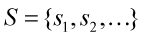
Let's assume they are taken at the intervals and are of the same size. Let the width of each image be `W`.
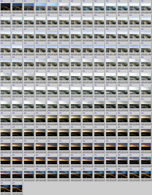
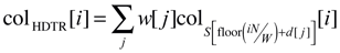
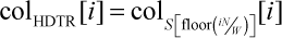
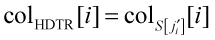
The HDTR image is formed by sampling columns (row-dominant sampling is very similar) from the set `S` as follows
This equation describes the following recipe. The width of the HDTR image canvas, `W`, which is the same as the width of each of the input images, is divided up into `W/N` strips. Each strip is be sampled from a different input image: column i of the HDTR is assigned from column i of the image indexed by iN/W.
For example if we had 5 images, each 20 pixels wide, then the sampling would be as follows.
| column | 0 | 1 | 2 | 3 | 4 | 5 | 6 | 7 | 8 | 9 | 10 | 11 | 12 | 13 | 14 | 15 | 16 | 17 | 18 | 19 |
| sampled from | 0 | 0 | 0 | 0 | 1 | 1 | 1 | 1 | 2 | 2 | 2 | 2 | 3 | 3 | 3 | 3 | 4 | 4 | 4 | 4 |
Generally, you'll have much larger input images (e.g. 1000 pixels in width) and more of them (e.g. 100), but the principle is the same.
temporal blending
If the individual images were taken with automatic exposure, the field brightness may vary from image to image. If the brightness difference across images is extreme, they it may be easier to normalize them upfront. I have not tried this route yet, so I will not say more aobut it.
In general, automatic exposure can lead to excessive banding that is difficult to correct. One of the charm of HDTR images is the varying light conditions seen across the frame. If the camera is performing its own corrections, it is not possible to separate exposure changes from differences in ambient light. A sophisticated approach might involve parsing the EXIF data from each image, calculating the exposure EV value and then normalizing the images to some baseline.
All this is to say that when the time-lapsed images are composited without any blending, the HDTR image will show heavy banding. To mitigate the undesirable effect, weighted averaging can be done from time-neighbouring frames. This is is called temporal blending because for a given column of the HDTR image we are sampling from the same column of images from different times. For example, column i in the HDTR is sampled not only from column i of image iN/W (e.g. 4:45pm) but also from column i of time-adjacent images (e.g. 4:40pm and 4:50pm).
Suppose we use the following set of weights: 1 2 4 2 1. The values for w[j] and d[j] in the equation above are
| j | 0 | 1 | 2 | 3 | 4 |
| d[j] | -2 | -1 | 0 | 1 | 2 |
| w[j] | 0.1 | 0.2 | 0.4 | 0.2 | 0.1 |
Thus column `i` is sampled from corresponding column of images `i_{N/W-2} ... i_{N/W+2}`, with each of the images weighted more heavily for image `i_{N/W}`.
The larger the number of weights, the smoother the resulting image. Compare a rough HDTR with a smooth HDTR.
Temporal blending has several disadvantages. Primarily, it dilutes the gradients in light conditions (lowers time contrast) that make HDTR images so interesting. At dawn, for example, there can be quite a substantial change in brightness and colour temperature from before sunrise to just after sunrise. If your frames started very close to sunrise, and if you blend the frames temporally, you may dilute the first frame with too much subsequent frames and reduce the brightness difference. On the other hand, if you have sampled a long time interval before and after the sharp change in light, temporal blending may be helpful.
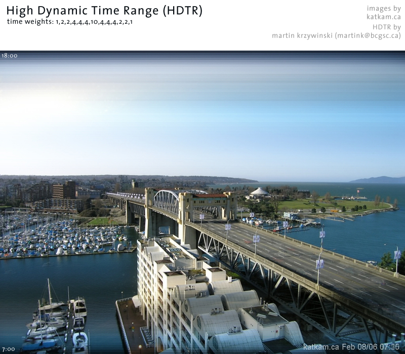
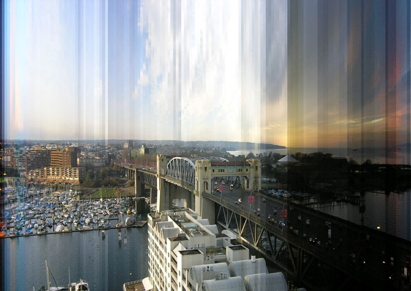
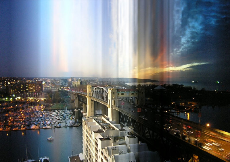
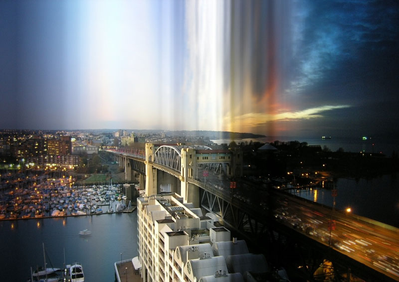
HDTR images of Burrard Bridge
I constructed HDTR images using images from katkam.ca, which are taken every 5 minutes from 7:00 to 18:00. A day is represented in a set of 133 images. The images were blended using a variety of temporal weights, as described above. In these HDTRs, time flows from left to right. The sun rises on the left and sets on the right. These represent my first attempts at HDTR images. They're not the best images, but I think they successfully illustrate the effect of temporal blending. Notice the decreased contrast across the strips in the edges of the heavily blended image.
|
no blending 
|
1,2,1 blending (15min) 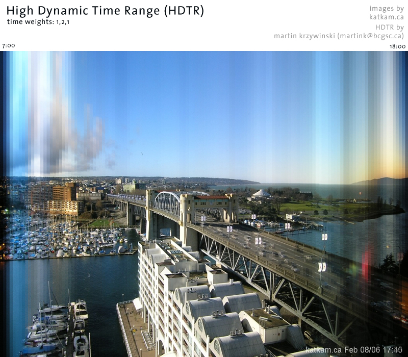
|
|
1,2,5,2,1 blending (25min) 
|
1,2,2,4,4,4,10,4,4,4,2,2,1 (80min) blending  |
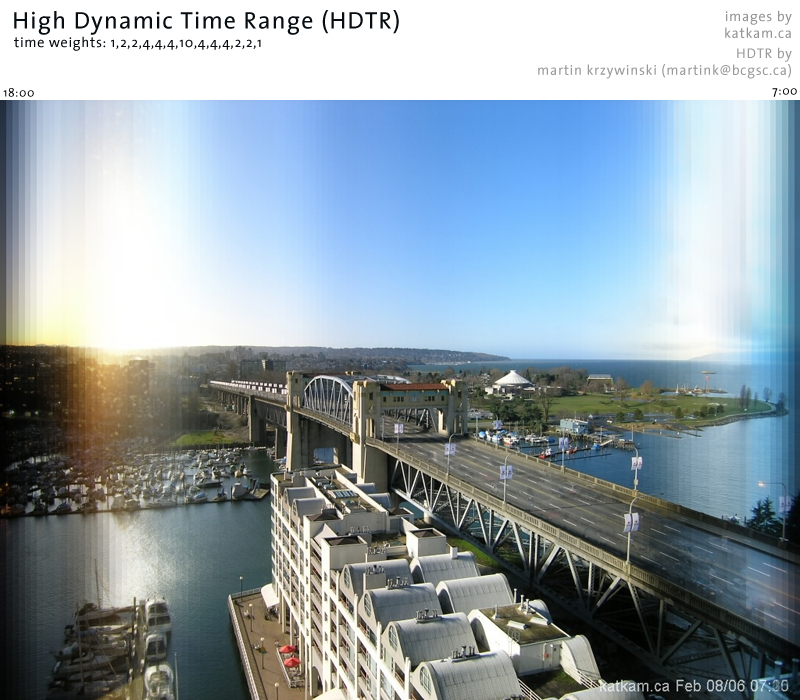
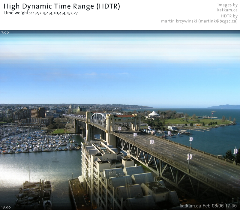
direction of time flow
The HDTRs below illustrate different directions of the flow of time across the image. All images are blended with long range averaging (weights 1,2,2,4,4,4,10,4,4,4,2,2,1).
|
|
|
|
 |
extending the golden hour
As I mentioned above, what makes HDTR images so interesting is the variation in light conditions across the time-lapse images. Light conditions can change quickly at dusk and dawn and if your images are taken at equal intervals you may have only a handful of images that sample this change. If all of the time-lapse images contribute equally to the HDTR image, the interesting times of day, from a lighting point of view, will have poor representation in the image.
Therefore, to keep things visually interesting it is desirable to accentuate the change in lighting condition in the HDTR image by extending the contribution of the images taken during this time. The two images below illustrate this principle. The image on the left contains equal contributions from each input image. The image on the right contains greater relative contributions from images taken early and late in the day.
Suppose you have 100 images in your time-lapse set. As described above, the ith column of the HDTR image is derived from the image indexed by `i_{N/W}`.
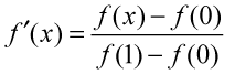
To extend the contribution of the images at the start and end of the time-lapse set, the image index `i_{N/W}`, which is linear with `i` is computed in another way. Using the logistic function, a new index is computed,
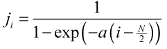
The function is normalized so that the domain and range extend over the same values.
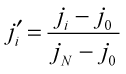
The HDTR image is sampled using the remapped index.
|

|
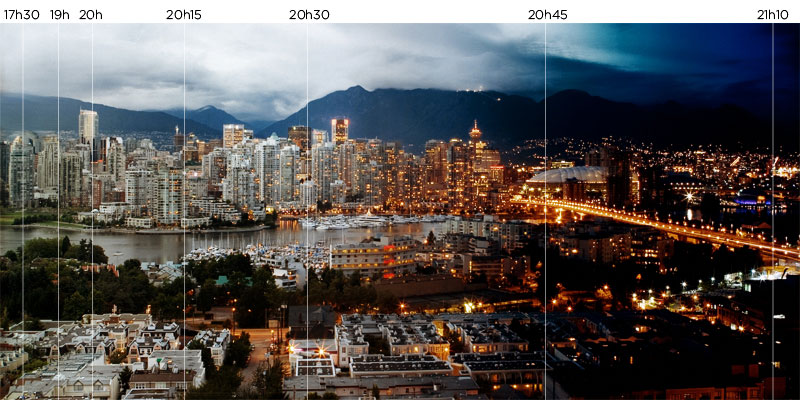
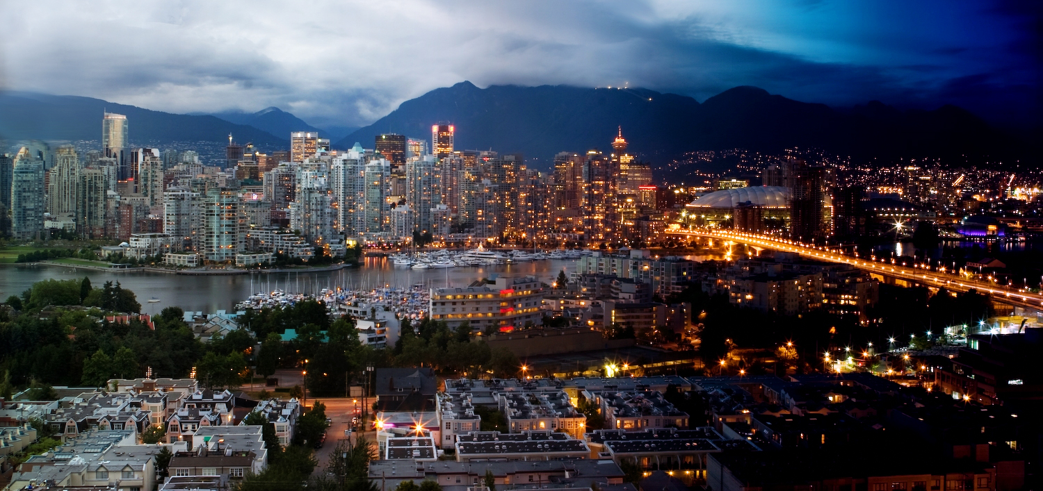
The time-lapse images for this example were taken every 5 minutes, except for the last hour of the day, when they were taken every 1 or 2 minutes.
spatial blending
When the contribution from any one image is large (such as in the case above, right), the banding pattern in the HDTR image is accentuated. Applying the time-blending described above decreases banding (below, left) but not entirely. To decrease banding further, spatial blending can be applied (below, right), a process in which the strips sampled from across the time-lapse frames are themselves blended with their immediate neighbours to smooth out the gradient. Temporal blending and spatial blending are closely related, but the difference is that during spatial blending one samples different input images with the same weight across a strip, and during temporal blending the weights are adjusted across the strip.
|
|
The spatial blending algorithm used to generate the image above (right) is similar to the temporal blending. Adjacent strips are blended over a distance
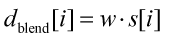
where s is the strip width and w is the fraction of the strip over which blending is done. Thus, given adjacent strips `s[i]` and `s[i+1]` sharing a boundary at `B`, the blending area is

At any position, `x` within this area the image pixel is sampled from images belonging to both strips in proportion to the distance from the boundary.
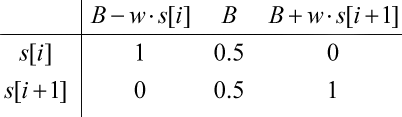
Thus at `B-wS[i]` image pixels are derived entirely from strip `S[i]`, at the boundary the pixel values are made up of equal components of strip `S[i]` and strip `S[i+1]`. At `B+w*S[i+1]` the contribution is from strip `S[i+1]` only.
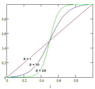
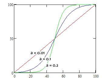
In the right image above, the blending weight `w_i` is determined according to the logistic function,
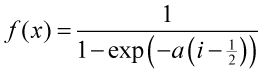
The best set of values of the blending distance and `a` is determined empirically for a given set of time-lapse images. The normalized value `g(x)` (`x=0..1`, `g(x)=0..1`) is shown below for `a = 1, 10, 20`.