thermodynamics
+ art
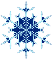
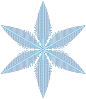
It's Snowing in my CPU — a Snowflake catalogue
Now she was round and as pure as the morning light, crystal clear and like a tiny silver mirror she was able to catch and give back every colour in the world about her.
— Paul Gallico, Snowflake
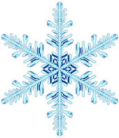
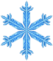
Somewhere in the world, it's snowing. But you don't need to go far—it's always snowing on this page. Explore random flurries, snowflake families and individual flakes. There are many unusual snowflakes and snowflake family 12 and family 46 are very interesting.
But don't settle for only pixel snowflakes—make an STL file and 3D print your own flakes!
Ad blockers may interfere with some flake images—the names of flakes can trigger ad filters.
And if after reading about my flakes you want more, get your frozen fix with Kenneth Libbrecht's excellent work and Paul Gallico's Snowflake.
In silico flurries: computing a world of snowflakes
High-resolution images from our Scientific American article In Silico Flurries: computing a world of snowflakes.
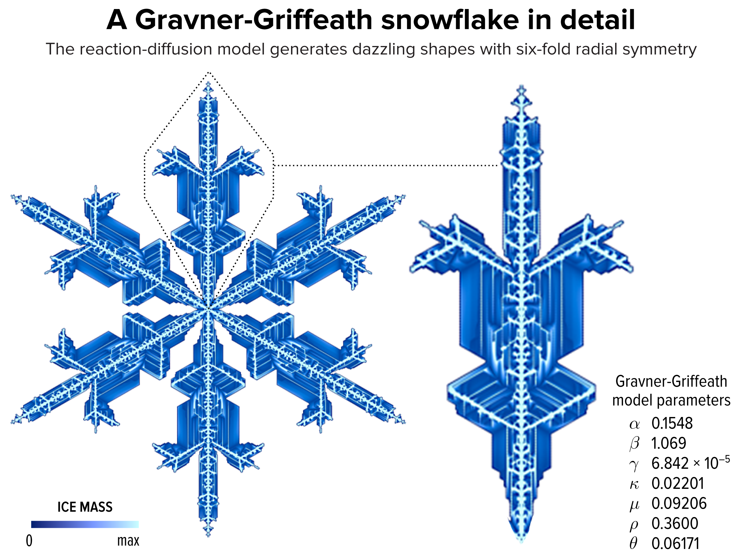
▲ Figure 1. An example of a snowflake grown using the Gravner-Griffeath model. Various amounts of ice (encoded by the blue tone) at different parts of the snowflake make up the six-fold radially symmetric shape.
(
zoom)
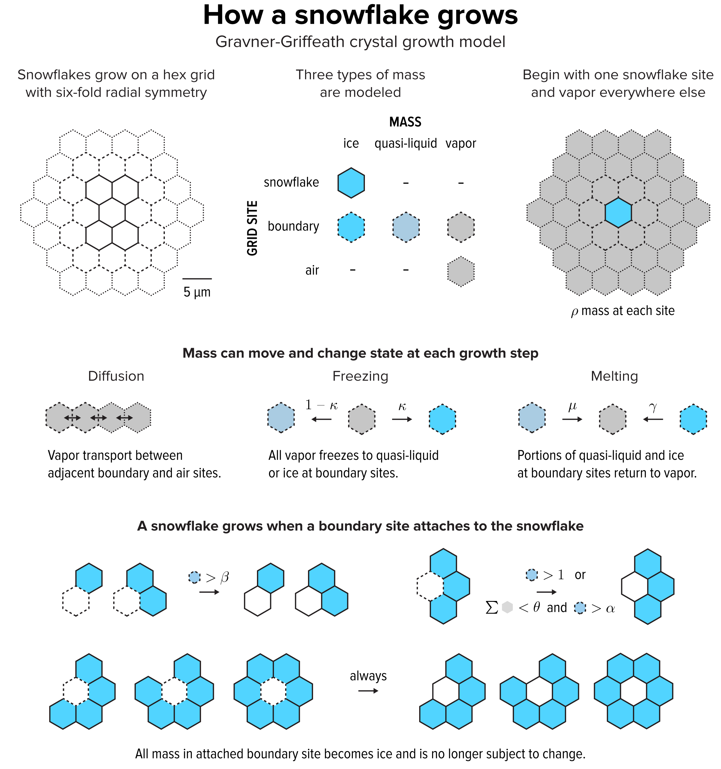
▲ Figure 2. The Gravner-Griffeath model is a type of reaction-diffusion system, with three kinds of “morphogens”: ice, quasi-liquid and vapor. The model is deterministic—given a set of parameters the output is always the same. Optionally the model can include randomness by perturbing the amount of vapor mass in every site at each step.
(
zoom)
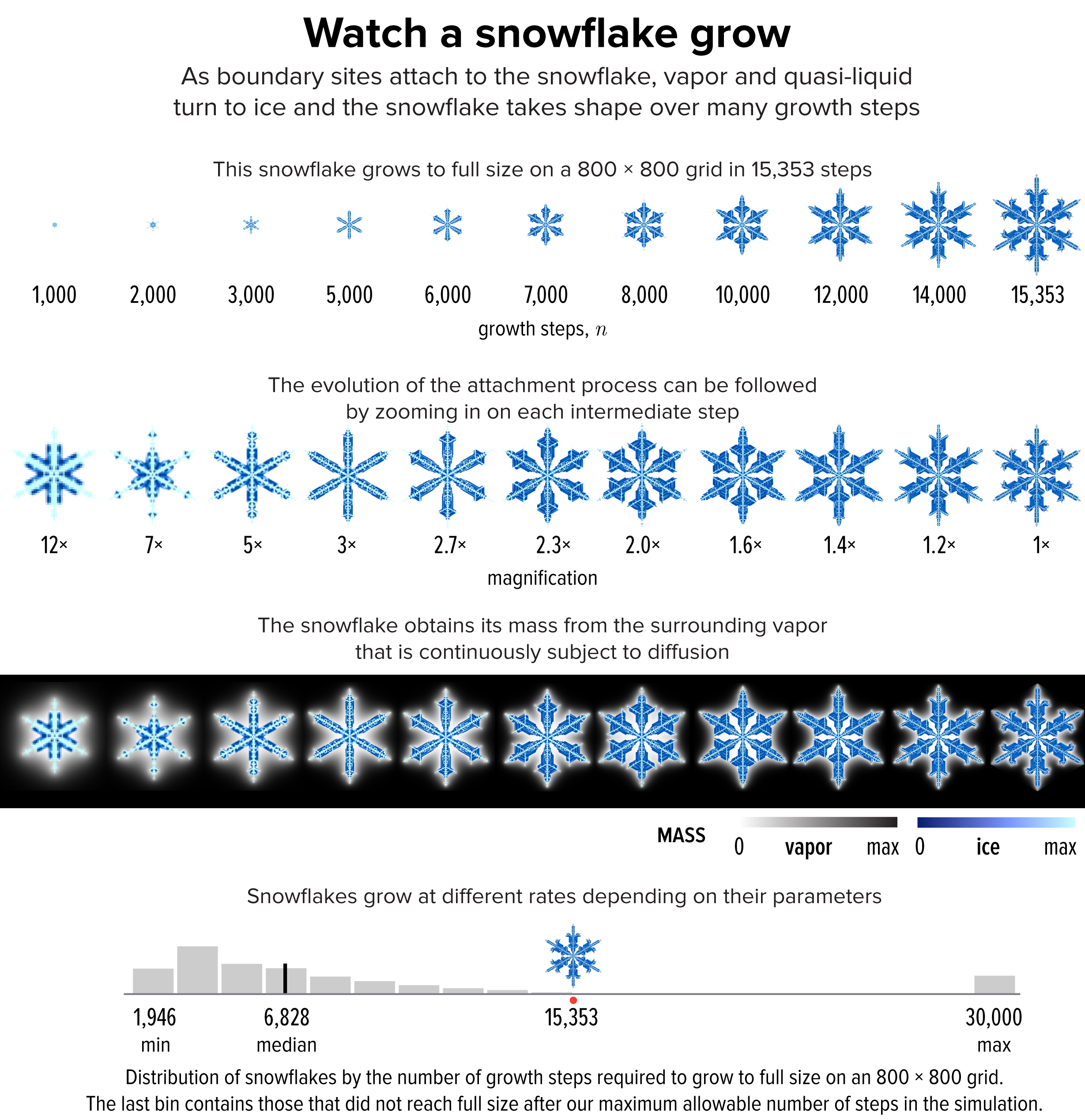
▲ Figure 3. The evolution of the snowflake from Figure 1 to full size at 15,353 growth steps.
(
zoom)
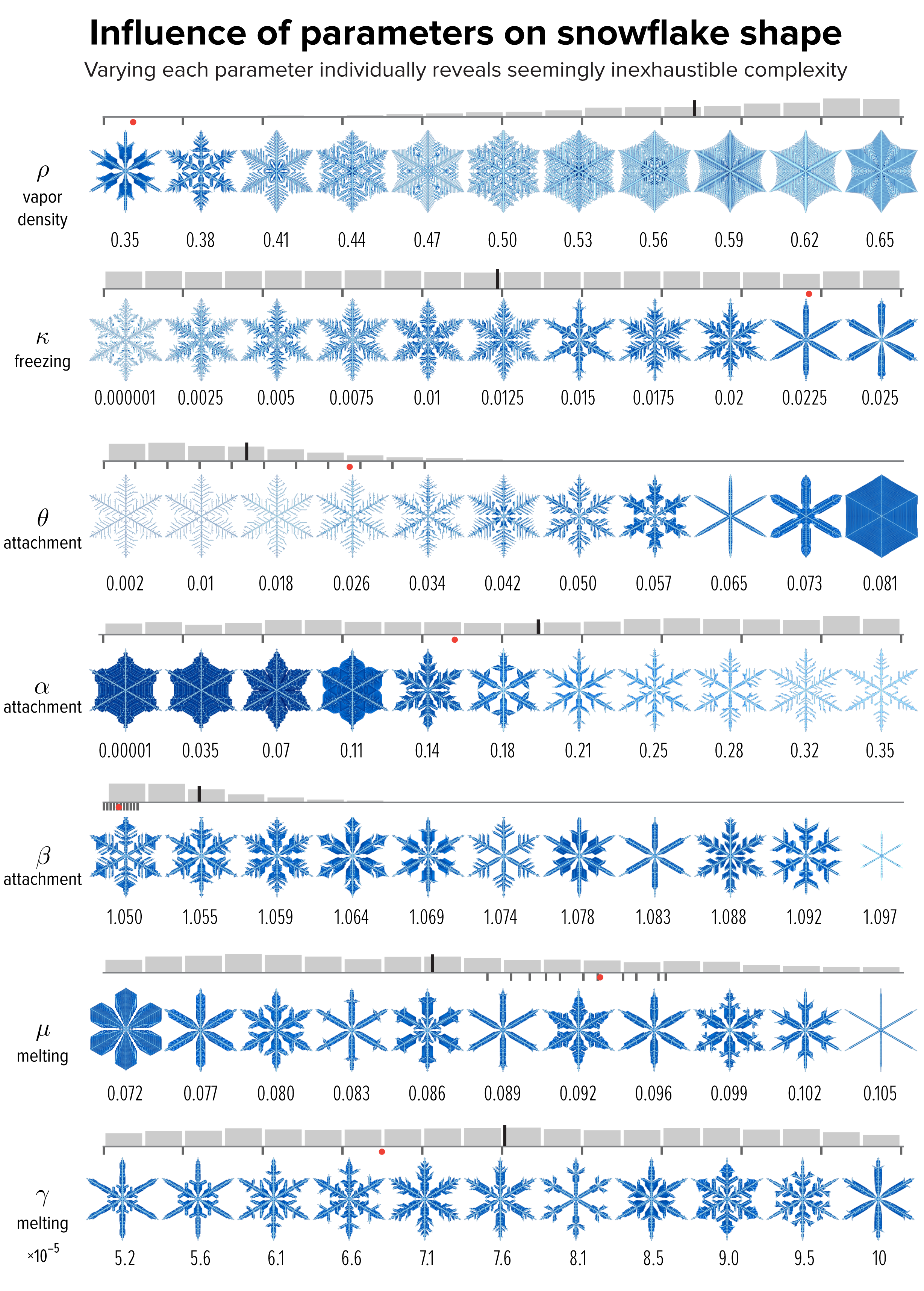
▲ Figure 4. The effect of varying each of the model parameters on the shape of the snowflake in Figure 1, whose parameter value is shown as a red dot. The images sample the parameter values shown by small black ticks. The distribution of snowflakes in our collection by parameter value is shown as a gray histogram. The median is the long black line among the bins.
(
zoom)
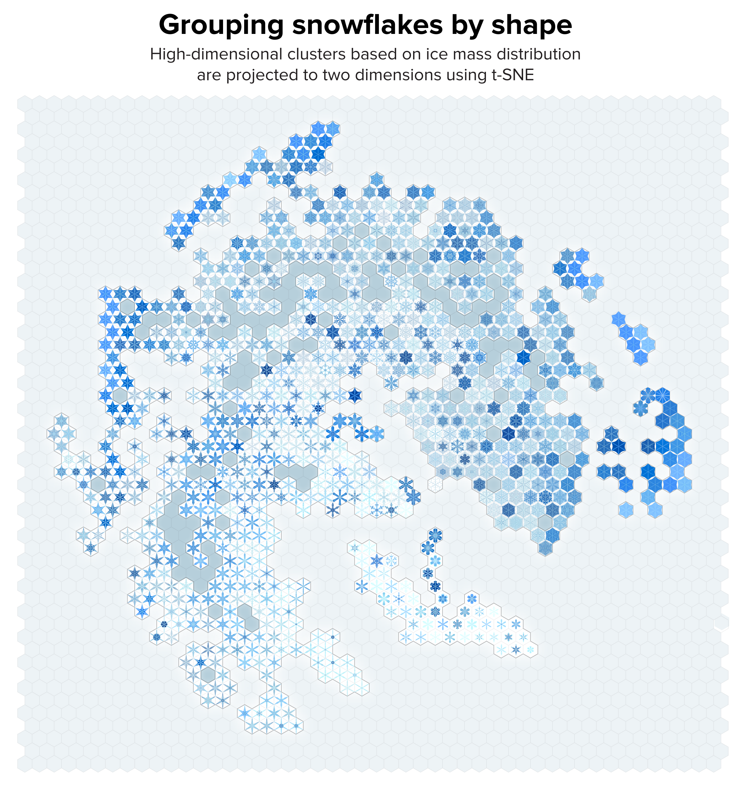
▲ Figure 5. Our collection of snowflakes clustered based on structural similarity. Clusters are projected onto two dimensions using t-SNE. The snowflakes are themselves arranged on a hex grid to allow tighter packing.
(
zoom)
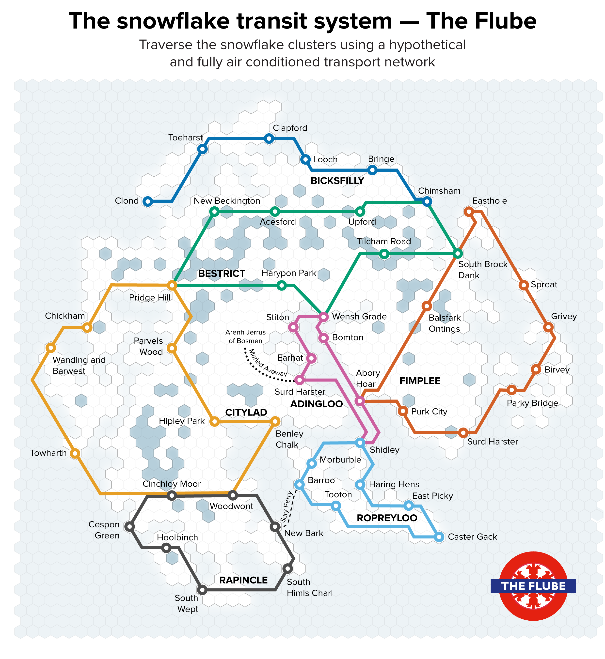
▲ Figure 6. A collection of paths in the two-dimensional t-SNE space of the snowflakes, affectionately named “The Flube.”
(
zoom)
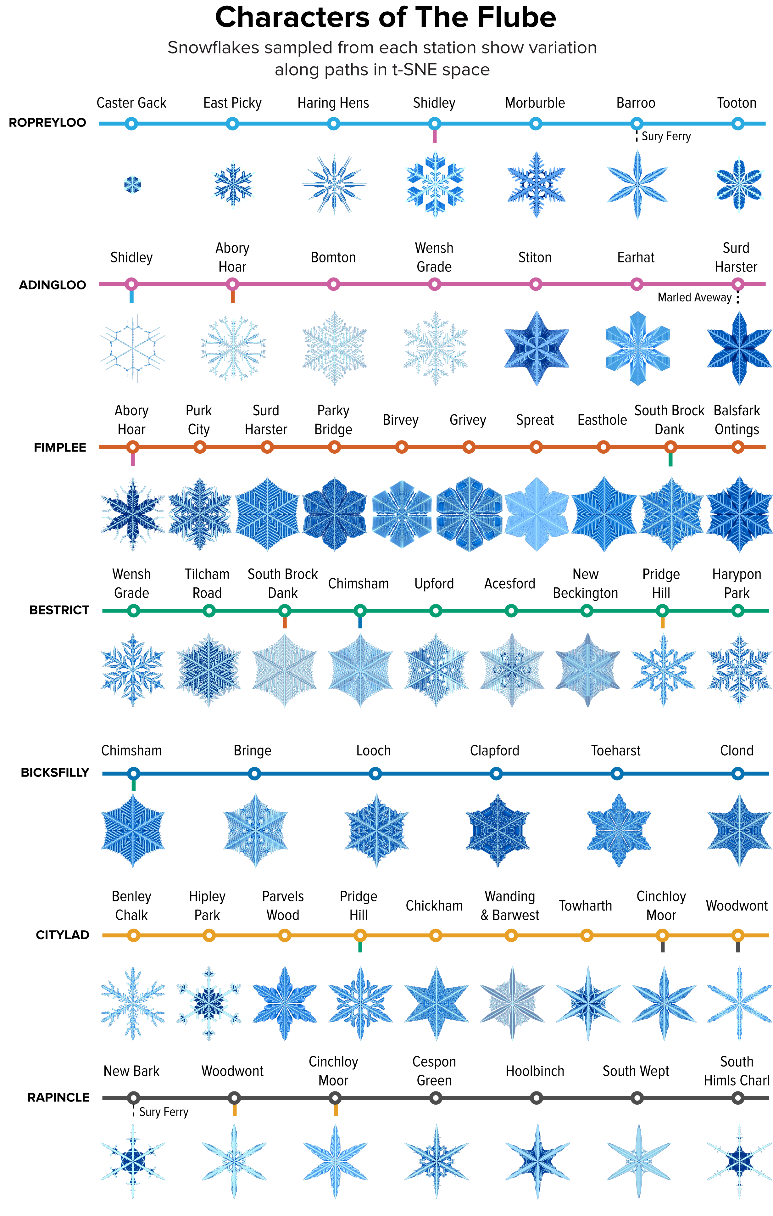
▲ Figure 7. A sample of the snowflakes found at the t-SNE hex grid of each station in The Flube, showing the variation in shape within and between clusters.
(
zoom)
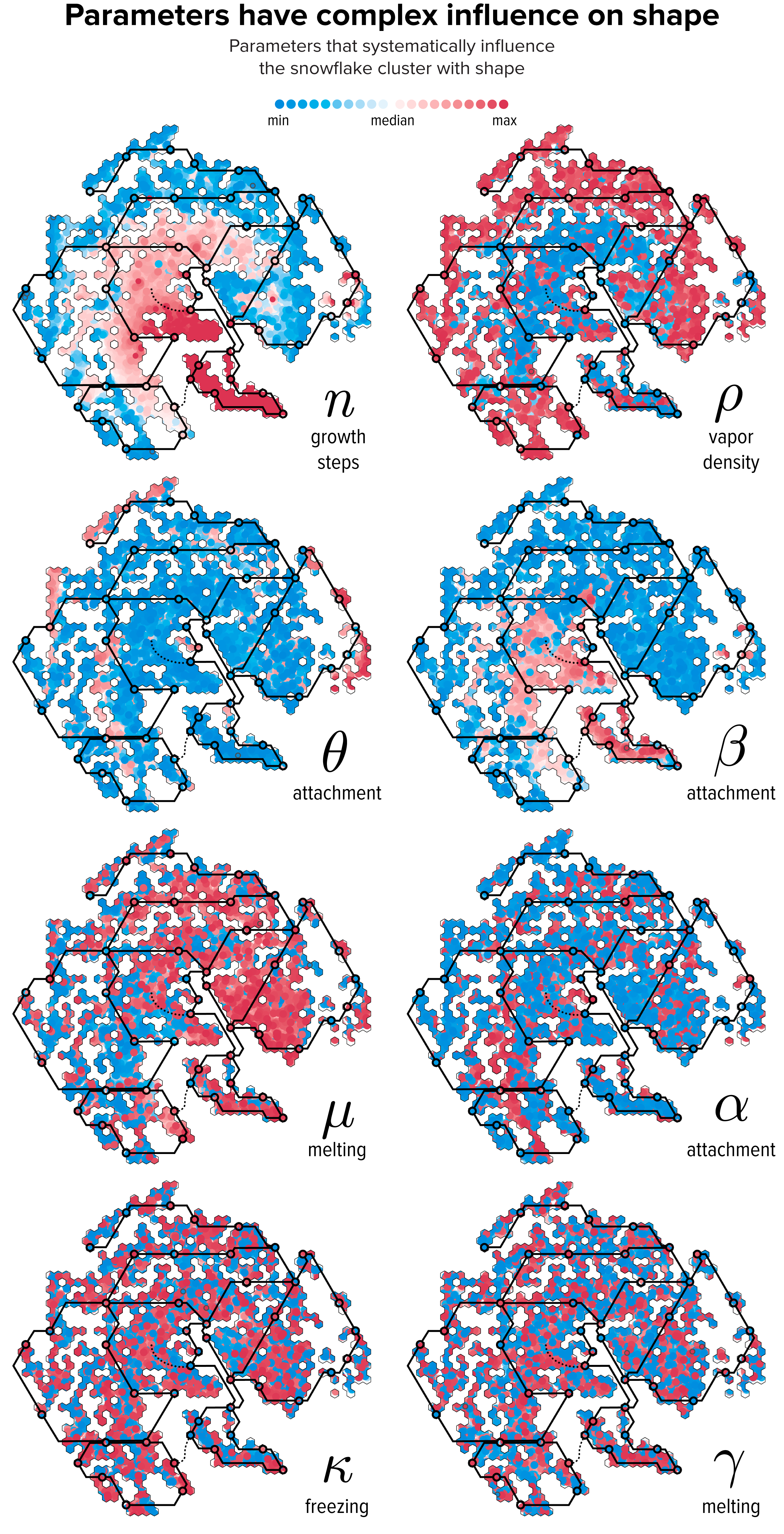
▲ Figure 8. The relationship between parameter values and t-SNE clustering. Each snowflake is drawn as a circle colored by the relative difference of the snowflake’s parameter with the median value. The lines of The Flube are superimposed to help interpret the variation in shape in Figure 7.
(
zoom)
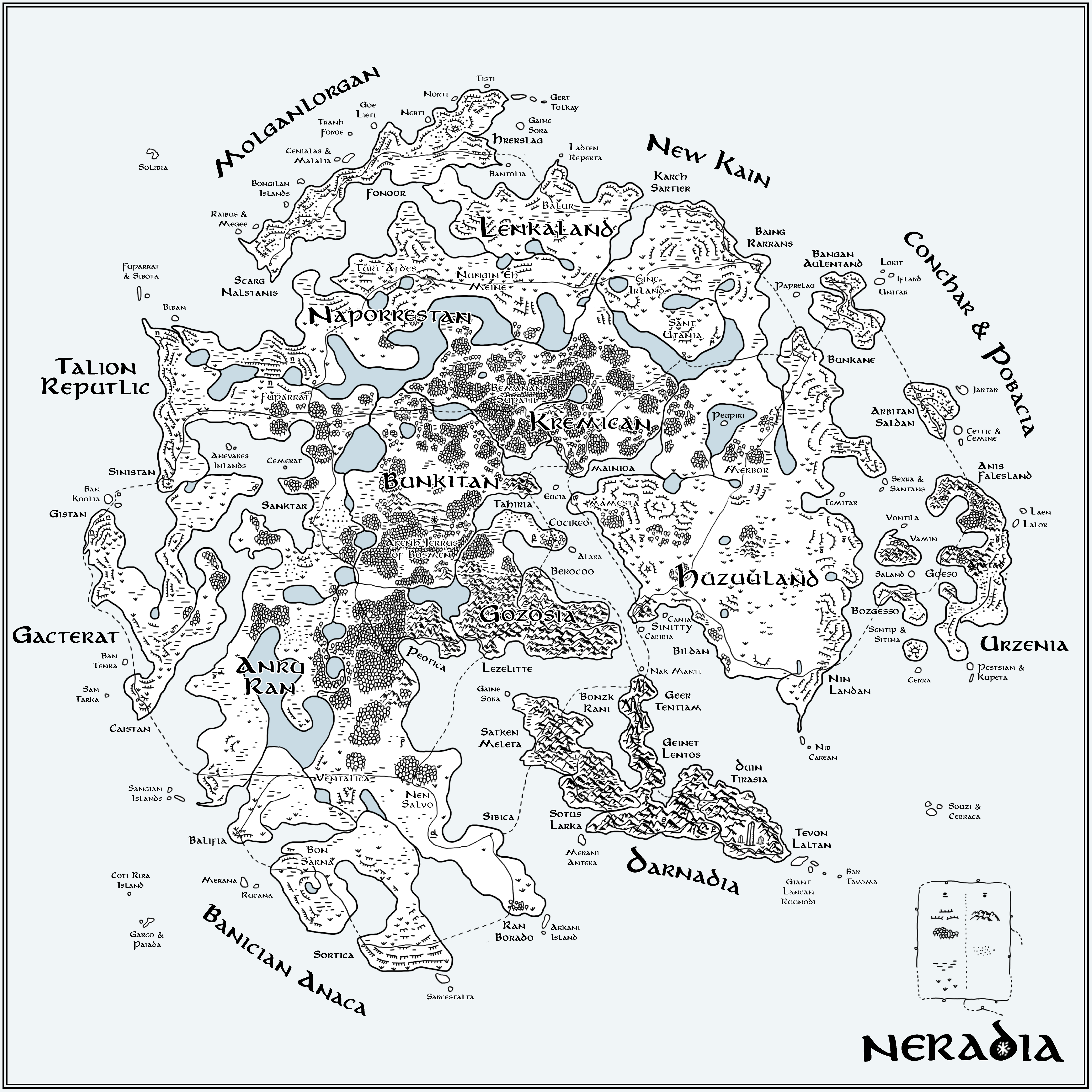
▲ Figure 9. A hand-drawn interpretation of the t-SNE map in Figure 5. Geographical features encode parameter values: woods (low ρ), grassland (low β), marsh (low μ) and desert (high θ). The speed at which the snowflake grew (steps to reach full size, n) is encoded by mountains (high n) and ice cliffs (low n). All names are generated using an RNN trained on 257 names of countries. The Flube network is drawn as thin lines with stations as loops with cities (medium size text) placed at the location of station positions in Figure 6.
(
zoom)