Learning Circos
Bioinformatics and Genome Analysis
Institut Pasteur Tunis Tunisia, December 10 – December 11, 2018
v2.00 6 Dec 2018 Download PDF slides
v2.00 6 Dec 2018
A 2- or 4-day practical mini-course in Circos, command-line parsing and scripting. This material is part of the Bioinformatics and Genome Analysis course held at the Institut Pasteur Tunis.
Quick links
BCGA 2018 | 1-day Circos course | Circos documentation best practices getting started | Brewer palette swatches | Color resources | Nature Methods Points of View Points of Significance
Circos case studies
Tuesday 11 December 2018 — Day 2
9h00 - 10h30 | Lecture 1 — Drawing the human genome
11h00 - 12h30 | Lecture (practical) 2 — Downloading and drawing human genes
14h00 - 15h30 | Lecture (practical) 3 — Downloading and drawing segmental duplications
16h00 - 18h00 | Lecture (practical) 4 — Creating an image montage
Concepts covered
drawing the human genome, karyotypes included in Circos distribution, generating random data with randomdata, heatmaps, color lists, interpolating colors with colorinterpolate, drawing human genes, drawing segmental duplications as links, creating image montages
Creating an image montage
In this final lecture, you'll be able to compare your answers from today's Lecture 2 and Lecture 3.
You'll also create a unique Circos poster as a sourvenir from the course.
Download Day 2 Lecture 4 Part 5 mosaic configuration and data.
Answers for challenge from Lecture 2.
karyotype = data/karyotype/karyotype.human.txt

<plots>
<plot>
type = histogram
file = track.gene.count.1mb.txt
r1   = 0.98r
r0   = 0.90r
fill_color = dgrey
stroke_thickness = 0

<rules>
<rule>
condition  = var(value) < var(plot_avg)
fill_color = red
flow       = continue
</rule>
<rule>
condition  = var(value) > var(plot_avg) + var(plot_sd)
fill_color = blue
flow       = continue
</rule>
<rule>
condition  = 1
value      = eval(sqrt(var(value)))
</rule>

</rules>

</plot>

<plot>
type = heatmap
file = track.gene.count.5mb.txt
r1   = 0.89r
r0   = 0.85r
color = spectral-9-div
stroke_thickness = 1
stroke_color     = white
</plot>

<plot>
type = tile
file = track.genes.txt
minsize   = 5u
r1        = 0.84r
r0        = 0.70r
margin    = 2u
thickness = 3p
padding   = 2p
stroke_thickness = 0
<rules>
<rule>
condition = var(name) =~ /^ZNF/
color     = red
</rule>
<rule>
condition = var(name) =~ /^SLC/
color     = black
</rule>
<rule>
condition = var(name) =~ /^FAM/
color     = grey
</rule>
<rule>
condition = 1
show      = no
</rule>
</rules>
</plot>

</plots>
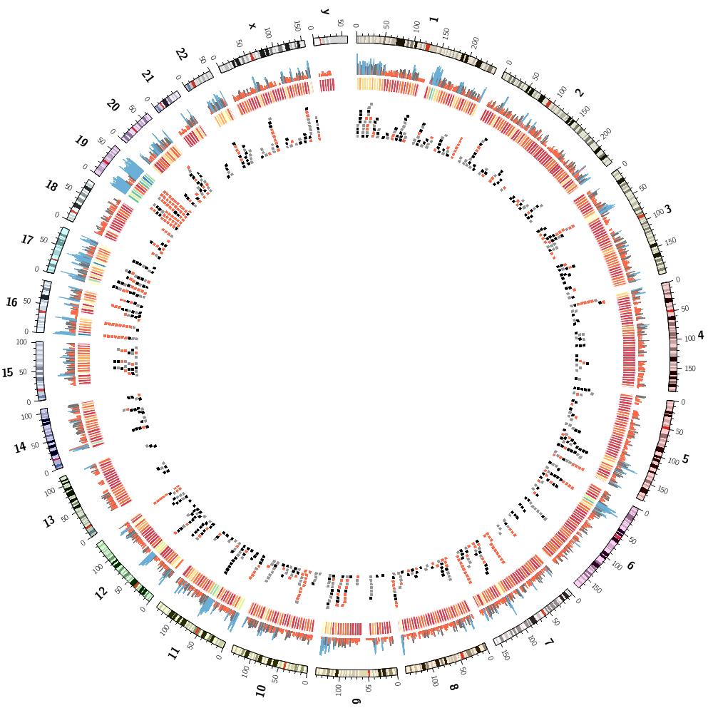
Answers for challenge from Lecture 3.
karyotype = data/karyotype/karyotype.human.txt

max_links* = 75000

<links>
<link>

record_limit = 10000

file = track.segdup.indexed.txt
bezier_radius = 0r
radius = 0.95r

<rules>
<rule>
condition = var(sizerank) > 500
show      = no
</rule>
<rule>
condition = var(sizerank) > 100
color     = black_a15
</rule>
<rule>
condition = 1
color     = eval(lc var(chr1))
#color     = eval(sprintf("spectral-9-div-%d",remap_int(var(size1),1000,100000,1,9)))
z         = eval(var(sizerank))
flow      = continue
</rule>
<rule>
condition = var(sizerank) < 10
thickness = 3
</rule>

</rules>
</link>
</links>
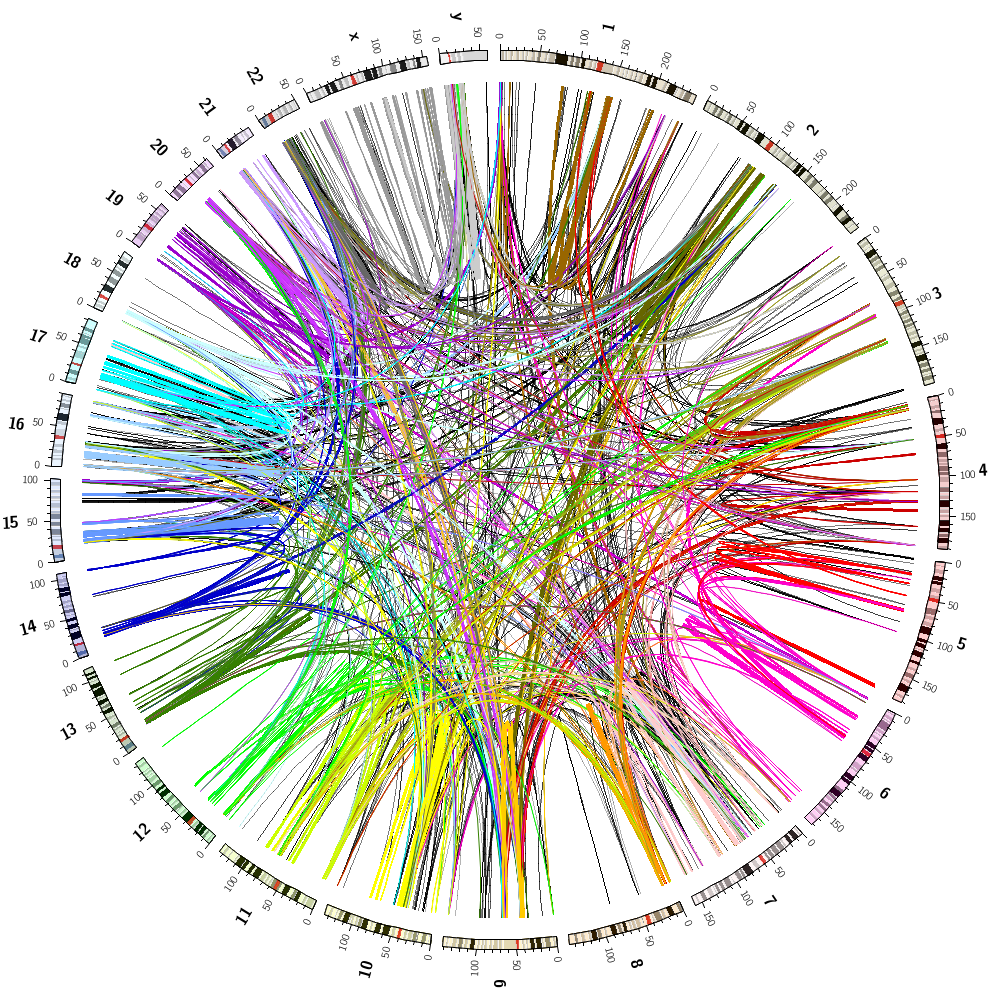
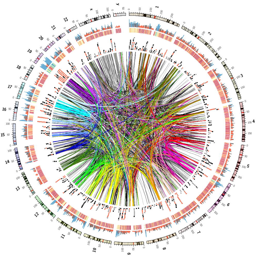
This image combines all track from Lectures 2 and 3.
karyotype = data/karyotype/karyotype.human.txt

<plots>
<plot>
type = histogram
file = ../1/track.gene.count.1mb.txt
r1   = 0.98r
r0   = 0.90r
fill_color = dgrey
stroke_thickness = 0

<rules>
<rule>
condition  = var(value) < var(plot_avg)
fill_color = red
flow       = continue
</rule>
<rule>
condition  = var(value) > var(plot_avg) + var(plot_sd)
fill_color = blue
flow       = continue
</rule>
<rule>
condition  = 1
value      = eval(sqrt(var(value)))
</rule>

</rules>

</plot>

<plot>
type = heatmap
file = ../1/track.gene.count.5mb.txt
r1   = 0.89r
r0   = 0.85r
color = spectral-9-div
stroke_thickness = 1
stroke_color     = white
</plot>

<plot>
type = tile
file = ../1/track.genes.txt
minsize   = 5u
r1        = 0.84r
r0        = 0.70r
margin    = 2u
thickness = 3p
padding   = 2p
stroke_thickness = 0
<rules>
<rule>
condition = var(name) =~ /^ZNF/
color     = red
</rule>
<rule>
condition = var(name) =~ /^SLC/
color     = black
</rule>
<rule>
condition = var(name) =~ /^FAM/
color     = grey
</rule>
<rule>
condition = 1
show      = no
</rule>
</rules>
</plot>

</plots>

max_links* = 75000

<links>
<link>

#record_limit = 10000

file = ../2/track.segdup.indexed.txt
bezier_radius = 0r
radius = 0.68r

<rules>
<rule>
condition = var(sizerank) > 500
show      = no
</rule>
<rule>
condition = var(sizerank) > 100
color     = black_a15
</rule>
<rule>
condition = 1
color     = eval(lc var(chr1))
#color     = eval(sprintf("spectral-9-div-%d",remap_int(var(size1),1000,100000,1,9)))
z         = eval(var(sizerank))
flow      = continue
</rule>
<rule>
condition = var(sizerank) < 10
thickness = 3
</rule>

</rules>
</link>
</links>
To finish off, let's make some random images based on this complex image that includes human genes and segmental duplications.
I've copied the configuration from the previous section but added a special rule to each block.
<rules>
<<include rule.hide.conf>>
...
</rules>
where the rule.hide.conf file is
<rule>
condition = rand() < conf(hidefraction)
show = no
</rule>
I have set hidefraction = 0.5 in circos.conf. Effectively, every data point has a 50% chance of being hidden.
You'll notice that for the links the rule is executed three times
<rules>
<<include rule.hide.conf>>
<<include rule.hide.conf>>
<<include rule.hide.conf>>
...
</rules>
This has the effect of increasing the possibilit of data being hidden to 1-0.5^3.
Let's make the image with this rule, but turn off the ideograms.
>circos -param ideogram/show=no -outputfile circos.1.png
Using the -param flag lets you dynamically overwrite any parameter values in the configuration. In the call above, the show parameter in the <ideogram> block is set to show=no, which basically turns of the display of ideograms.
The -outputfile sets the output filename.
You can change the fraction to hide on the command line using -param
>circos -param ideogram/show=no -param hidefraction=0.9 -outputfile circos.1.png
Finally, we're going to randomize all the colors (keeping black and white as they are).
>circos -param ideogram/show=no -param hidefraction=0.75 -outputfile circos.1.png -randomcolor white,black
Everyone's image will be different.
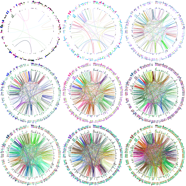
Let's make a set of 9 images, each with a different hiding fraction. Again, each one will be different because the colors are randomized as is the data hiding. I've set up a small batch file make.random that runs these four jobs in the background, which is achieved by the trailing &.
We will finally use Image Magick's utilities convert and montage to create a tiling of our images. See the make.tiles script for this.
As a challenge, try to replace one of your images with a photo of yourself, or any other image!
#!/bin/bash

OPT="-param ideogram/show=no -randomcolor white,black"
for i in `seq 1 9` ; do
f=`echo "scale=1;(10-$i)/10" | bc`
echo "drawing for hidden fraction $f"
circos $OPT -outputfile circos.$i.png -param hidefraction=$f &
done
#!/bin/bash

for i in `seq 1 9`; do
convert circos.$i.png -gravity Center -crop 850x850+0+0 circos.$i.crop.png
done

montage -mode Concatenate -geometry 850x850 circos.*.crop.png circos.tiles.png
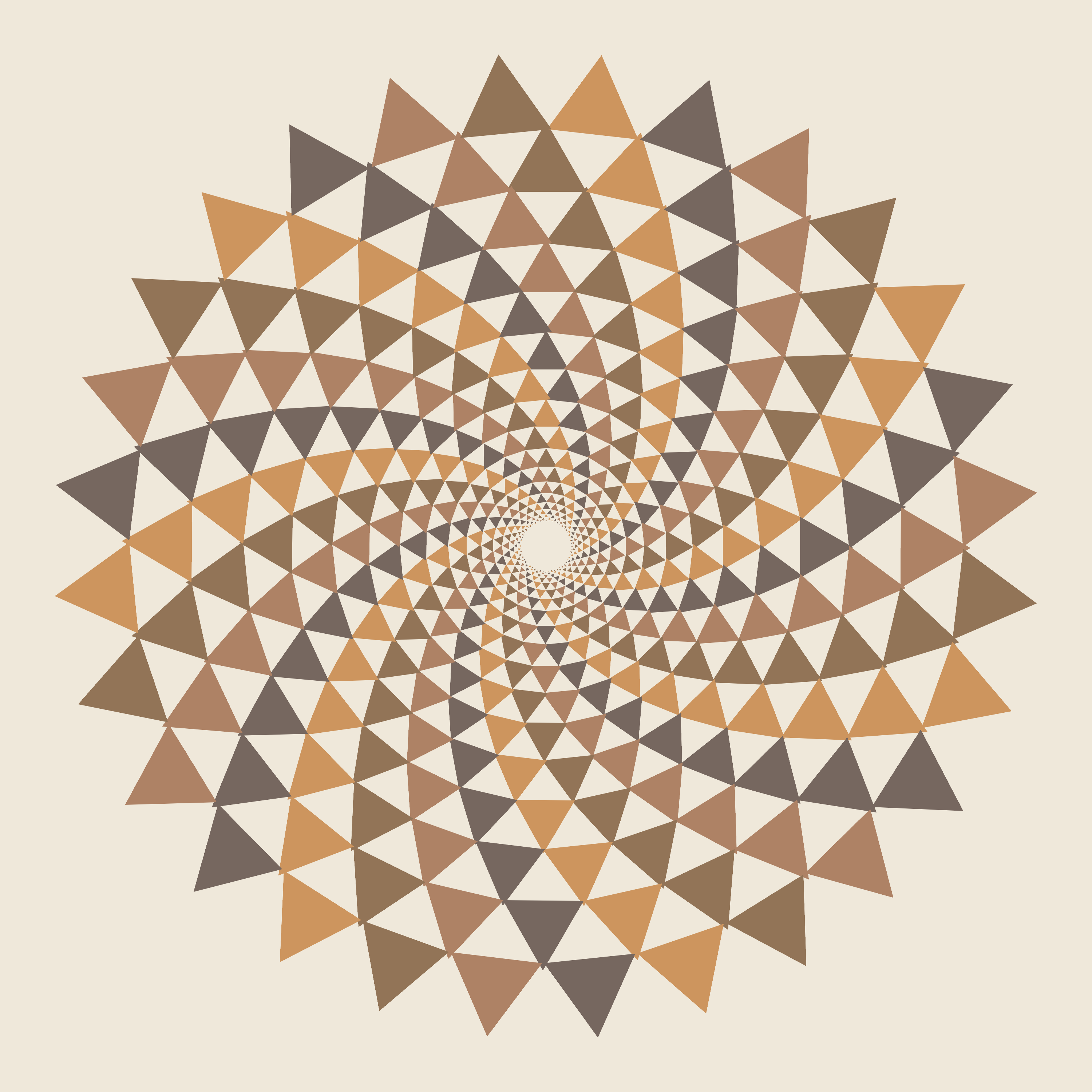
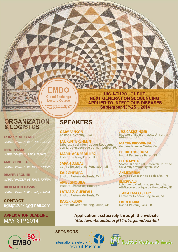
Creating a Tunesian mosaic based on the image used for the 2014 Bioinformatics and Genome Analysis Course poster and the colors on the tiles outside of the computer room in the Pasteur Institute in Tunis.
We won't be able to reproduce the image exactly because Circos can only draw equilateral triangles, which are one of the glyphs that can be used in a scatter plot.
For a source of colors from the image, let's use the tiles outside of the computer room. Below is a photo of those tiles (with surface blur applied to even out the colors).
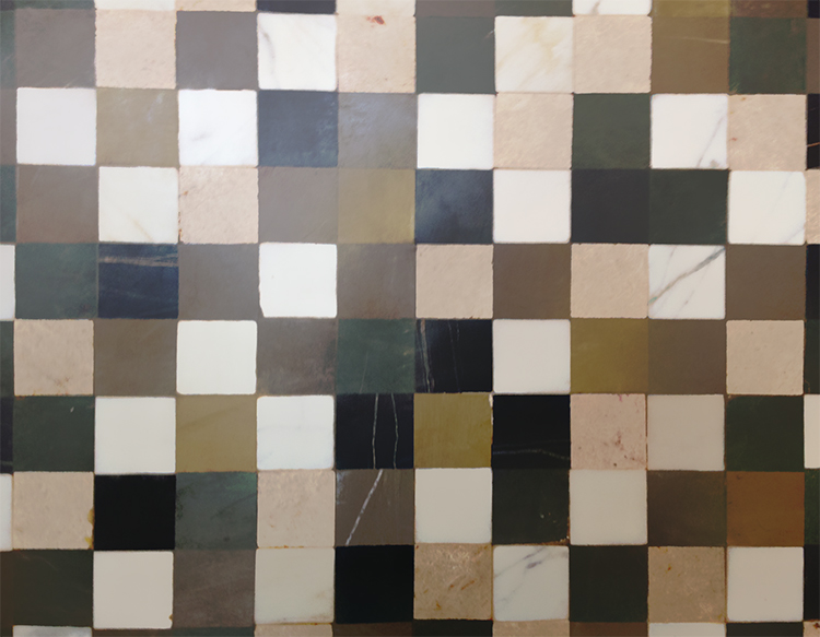
Here is a sampling of some of the colors in the photo.
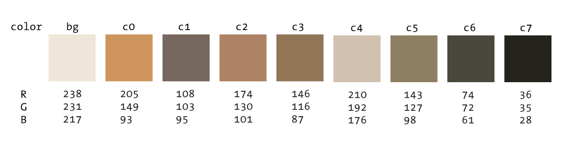
We'll define these colors in Circos by appending to the <colors> block. Because a large number of colors are already defined by default in this block, anytime you use this block, any contents will be appended.
<colors>
bg = 239,232,218
c0 = 205,149,94
c1 = 118,103,95
c2 = 174,130,101
c3 = 146,116,87
c4 = 210,192,176
c5 = 143,127,98
c6 = 74,72,61
c7 = 35,35,28
</colors>
The first thing we need to do is create the data files for each part of the image. There are three parts. Starting from the outside, a step line, small dashes, and the triangles.
The step line is going to be made with a histogram. We'll make a histogram with a black background and white outline.
The small dashes will be a highlight track for which we'll use rules to determine how densely the dashes are drawn.
Finally the triangles will be made from a scatter plot with glyph=triangle. The tricky part will be to resize the triangles and reposition them radially so that they create more-or-less the mosaic we're after. It won't be perfect, but close.
Create the track files.
 cd data
 ./make.all.tracks.sh
You'll see that this calls the make.track script, which, in turn, writes to files like scatter.0.txt, histogram.0.txt and highlight.0.txt. Here the 0 indicates the offset that determines where the element's start position is.
Take a look at the make.track script and read the comments in front of each section. Try to understand what is going on.
Initially, create the image with use=no in the <rules> block for the scatter plots. This will show you the original position of all the triangles, as defined by the make.track script.
Now start turning each rule on and redraw the image to see what the rule does. The key to the mosaic is coloring the triangles appropriately. We want the color to be offset by one position for adjacent layers.
Once you've activated all the rules, activate the second scatter plot track in circos.conf. Do you like this version better? Then activate the histogram and highlight tracks.
Try to make your image different from everyone. Here are a few things to experiment with.
Toggle any of the tracks off if you prefer a simpler image.
Redefine the colors, maybe adding a vivid blue.
Change how the color indexes are assigned to the layers. For example, this rule will cycle between colors c0..c3 because we're taking modulo 4 of the value based on the id and layer.
color = eval(sprintf("c%d",( var(id) - int((var(layer)+1)/2) ) % 4))
If you look carefully at the spiral, you can figure out the color scheme. Track the triangle that is orange with color c0.
 layer  color
 0     [0]1 2 3 0 1 2 3 0 1 2 3 0
 1      3[0]1 2 3 0 1 2 3 0 1 2 3
 2      3[0]1 2 3 0 1 2 3 0 1 2 3
 3      2 3[0]1 2 3 0 1 2 3 0 1 2
 4      2 3[0]1 2 3 0 1 2 3 0 1 2
 5      1 2 3[0]1 2 3 0 1 2 3 0 1
 6      1 2 3[0]1 2 3 0 1 2 3 0 1
 7      ...
The second term int((var(layer+1)/2)) makes sure that the index assignment is the same between adjacent layers after layer 1. See the script data/showindex, shown below, which implements this rule and shows you the color index.
use strict;
for my $layer (0..10) {
    my @colors;
    for my $id (0..15) {
      my $color = ($id - int( ($layer+1)/2 ) ) % 4;
      push @colors, $color;
    }
    print join(" ",@colors)."\n";
}
> data/showindex
0 1 2 3 0 1 2 3 0 1 2 3 0 1 2 3
3 0 1 2 3 0 1 2 3 0 1 2 3 0 1 2
3 0 1 2 3 0 1 2 3 0 1 2 3 0 1 2
2 3 0 1 2 3 0 1 2 3 0 1 2 3 0 1
2 3 0 1 2 3 0 1 2 3 0 1 2 3 0 1
...
Find a way to change the rule so that the spirals turn counterclockwise.
Change the rate at which colors are randomly adjusted. At what point can you no longer perceive the spirals.
Generate mosaics of different colors and compose them using the montage tool. See section 4 of this lecture and the script (../4/make.tiles) to see how to use montage.
What happens if you cange the glyph to square or circle?
open(F,">histogram.$CONF{offset}.txt");
for my $i ( 1 .. 5*$CONF{len}/$CONF{div} ) {
  my $bin   = $CONF{len}/$CONF{div}/5;
  my $start = ($i-1)*$bin;
  my $end   = $start + $bin - 1;
  printf F ("%s %d %d %f type=histogram\n",
            $CONF{axisname},
            $start,$end,
            $i % 2 ? 1 : 0.5);
}
close(F);

# Highlight track
open(F,">highlight.$CONF{offset}.txt");
for my $i ( 1 .. $CONF{len} ) {
  my $start = ($i-1);
  my $end   = $start+1;
  printf F ("%s %d %d\n",
            $CONF{axisname},
            $start,$end);
}
close(F);

# Make the scatter plot track - these will be the triangles
# iterate across layers
open(F,">scatter.$CONF{offset}.txt");
for my $layer (1..$CONF{layers}) {

  my $id = 0;

  # iterate across divisions in this layer
  for my $i (1..$CONF{div}) {

    # odd layers - triangles at odd positions
    next if ($layer % 2) && ($i % 2);

    # even layers - triangles at even positions
    next if ! ($layer % 2) && ! ($i % 2);

    # position along axis for this division
    my $pos = ($i-1+$CONF{offset}) * $CONF{len}/$CONF{div} % $CONF{len};;

    # report a point here, the value of the point is
    # the fractional layer number and we also
    # store the two parameters "id" (unique id per layer)
    # and the layer number
    printf F ("%s %d %d %.4f id=%d,layer=%d\n",
              $CONF{axisname},
              $pos,$pos,
              1-($layer-1)/$CONF{layers},
              $id,$layer-1);
    $id++;
  }

}
#!/bin/bash

LAYERS=20

./make.track -layers $LAYERS -offset 0
./make.track -layers $LAYERS -offset 1
for my $layer (0..10) {
    my @colors;
    for my $id (0..15) {
      my $color = ($id + int( ($layer-1)/2 ) ) % 4;
      push @colors, $color;
    }
    print join(" ",@colors)."\n";
}
<plot>

type  = scatter
glyph = triangle
file  = data/scatter.counter(plot).txt
Scatter plot glyphs are automatically rotated so that they always point into the circle. The angle_shift parameter adds to this angle.
#angle_shift = 45

glyph_size  = 30
The value of each scatter point was a fractional layer index in the range [0,1]. This is the "y-value" of the point.
min   = 0
max   = 1

r1    = 0.90r
r0    = 0.05r
There are two things we have to do for each point:
1. assign a color to the triangles so that glyphs that are off by one index in adjacent layer pairs have the same color, thereby giving the mosaic a spiral look 2. change the size of the glyph based on layer number, so that glyphs shrink closer to the inside of the circle
# layer  color index
# 0      1 2 3 0 1 2 3 0 1 2 3 0
# 1      0 1 2 3 0 1 2 3 0 1 2 3
# 2      "
# 3      3 0 1 2 3 0 1 2 3 0 1 2
# 4      "
# 5      2 3 0 1 2 3 0 1 2 3 0 1
# 6      "

<rules>

#use   = no

flow  = continue
We've made two scatter point tracks, one with offset 0 (scatter.0.txt) and one with offset 1 (scatter.1.txt). We've defined the file to use based on the plot counter. So if the counter is 0, we're using scatter.0.txt
These rules check which offset we are using and apply a different rotation for the glyphs and different color cycle. Changes the size of the triangles based on value
<rule>
condition   = 1
glyph_size  = eval(remap_int(var(value)**2.5,0,1,1,250))
</rule>
Changes colors for first scatter plot
<rule>
use = no
condition   = counter(plot) == 0
angle_shift = 0
color       = eval(sprintf("c%d", ( var(id) - int((var(layer)+1)/2) ) % 4))
</rule>
Changes colors for second scatter plot (alternating triangles)
<rule>
use = no
condition   = counter(plot) == 1
angle_shift = 0
color       = eval(sprintf("c%d", 4 + ( var(id) - int((var(layer)+1)/2) ) % 4))
</rule>
Randomly changes colors of ~5% of the triangles
<rule>
use = no
condition   = rand() < 0.05
color       = eval(sprintf("c%d",int(1+rand(8))))
</rule>
Repositions the triangles closer to the center.
<rule>
use = no
condition   = 1
value       = eval(var(value)**3.2)
</rule>

</rules>

</plot>
chromosomes_units = 1
karyotype         = data/scale.txt

<plots>

<<include scatter.conf>>
<<include scatter.conf>> <<include histogram.conf>> <<include highlight.conf>>
</plots>

<colors>
bg = 239,232,218
c0 = 205,149,94
c1 = 118,103,95
c2 = 174,130,101
c3 = 146,116,87
c4 = 210,192,176
c5 = 143,127,98
c6 = 74,72,61
c7 = 35,35,28
</colors>

<image>
<<include etc/image.conf>>
background* = bg
svg*        = no
</image>

<<include ideogram.conf>>
<<include etc/colors_fonts_patterns.conf>>
<<include etc/housekeeping.conf>>