A 2- or 4-day practical mini-course in Circos, command-line parsing and scripting. This material is part of the Bioinformatics and Genome Analysis course held at the Institut Pasteur Tunis.

Quick links

BCGA 2018 | 1-day Circos course | Circos documentation best practices getting started | Brewer palette swatches | Color resources | Nature Methods Points of View Points of Significance

Concepts covered

drawing the human genome, karyotypes included in Circos distribution, generating random data with randomdata, heatmaps, color lists, interpolating colors with colorinterpolate, drawing human genes, drawing segmental duplications as links, creating image montages

You're now pretty much ready to work on small projects on your own.

In this lecture, you'll download and draw human genes. You'll find answers to this challenge in Lecture 4.

Download human gene data set

Download the NCBI RefSeq gene set from the UCSC genome browser table viewer.

 clade:    Mammal
 genome:   Human
 assembly: Dec 2013 (hg38)
 group:    Genes and Gene Predictions
 track:    NCBI RefSeq
 table:    RefSeq Curated

To learn about the format of this file, click on "Describe table schema".

I encourage you to download the file yourself but if the network connection is slow, you can find it in day.2/data/genes.human.refseq.txt.

Create a gene short list

Create a version of the gene file whose lines do not match ANY of these patterns:

 random
 _alt
 none
 chrUn

You can do this by repeatedly piping to grep

cat file.txt | grep -v random | grpe -v _alt | ...

or use alternation

cat file.txt | grep -v "random\|_alt\|..."

This should yield about 43,000 genes.

Now filter this list further to accept genes with unique values for the name2 field. This is the field in this column

 cat ../../data/genes.human.refseq.txt | awk '{print $13}'

You can do this by first sorting by this field with the -u flag. Alternatively, you can generate a version of each line with this field at the start of the line and then applying sort -k 1,1 -u.

 cat ../../data/genes.human.refseq.txt | awk '{print $13,$0}'

There are about 19,300 genes with unique names. Use this list.

If you want an even shorter list, use uniq -w 3 to consider only the first 3 letters in the gene name when calculating unique names, once you have the name field in the first column.

Calculate some statistics

Use the histogram script, for details see Day 4 Lecture 4, to generate a distribution of gene sizes.

For this, you'll want to parse the file with something like awk, extract the appropriate columns, calculate the size (e.g. transcription start to end) and then draw the histogram.

What is the average gene size? What about the 50% percentile?

Count the genes per chromosome

Use sort and uniq to count the number of genes on each chromosome.

Create gene track

Parse the gene file to generate a Circos data file appropriate for a highlight track. It should have the format

CHR START END NUM_EXONS name=GENENAME

The number of exons is one of the fields in the file.

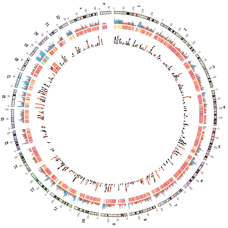
Draw gene regions

Use the resample Circos tool to generate a count of genes in 1 Mb windows. Use -bin 1e6 -count flags to do this.

Draw a Circos image with the gene counts as a histogram. Use the template provided in etc/ to get you started.

Draw the track again below the histogram as a line plot.

Draw the track again below line plot as a heatmap.

Use the histogram script to calculate the average number and standard deviation of gene counts. Write rules for each track that make all data points for which values are lower than average red and those with values higher than average+sd blue. Alternatively use the var(plot_avg) and var(plot_sd) notation in the rule condition.

Change the scale of the histogram to sqrt() by remapping the values in a rule block. Do this after the color rules described above. Also try log10 scale. You can remap the value of a data point using

<rule>
condition = 1
value = eval(sqrt(var(value)))
</rule>

Extract the first 3 characters from the names of the genes and tabulate their frequency distribution (use sort and uniq). What are the three most frequent 3 character prefixes? Create a tile track that shows only genes that match these and use a different color for each prefix (e.g. red, black, grey).

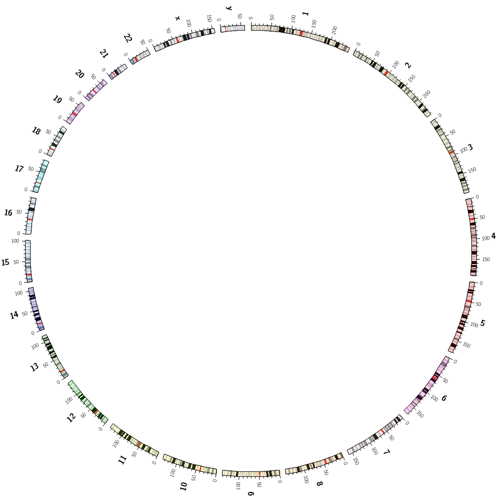
You're working towards an image like the one below.

karyotype = data/karyotype/karyotype.human.txt

Follow the instructions in above to populate the <plot> blocks.

#<plots>
#<plot>
#</plot>
#</plots>

▲ sessions/day.2/lecture.2/1/circos.png (zoom)