


fitness + math
`k` index: a crossfit and weightlifting benchmark
I want to diverge from my traditional scope of topics and propose a new benchmark for weightlifting and CrossFit: the `k` index.
The `k` index is brainy and fun and gives you a new way to structure your goals. At high values, it's very hard to increase, making each increment a huge challenge.
Going around with a t-shirt that says "`k=40` at everything" is maximally geeky and athletic.
definition of `k` index
For a given movement (e.g. squat, deadlift, press), you achieve index rank `k` if you can perform `k` unbroken reps at `k`% of your current one rep max (1RM).
Unbroken means no more than 1–2 seconds of pause between each rep. Exact standards would need to be established for competition.
example of `k` index
Suppose an athlete's one rep max (1RM) squat is 100 kg (220 lb).
The athlete will have a `k` index rating of `k=10` for squats if they can perform 10 unbroken reps at 10% 1RM, which is 10 kg (22 lb).
The athlete will have a `k` index rating of `k=20` for squats if they can perform 20 unbroken reps at 20% 1RM, which is 20 kg (44 lb).
The athlete will have an independent `k` index rating for other movements like deadlift and press. These ratings are likely to be different for each movement.
range of values
The minimum `k` index is `k=0` and it's a value we're born with.
The maximum theoretical `k` index is trivially `k=100` because, by definition, you cannot lift more than your current 1RM.
The maximum practical `k` index is much lower than `k=100` and probably in the range of `k = 50`.
expected `k` value
If you perform `r` reps at weight `w` you can estimate your 1RM using the Epley formula `w(1+r/30)` assuming `r>1`. In other words, for each rep at a weight `w` your estimate of your 1RM increases by ~3.3% above `w`.
There are various 1RM estimate equations and generally they are designed for fewer than 20 reps.
In some estimates, like by Mayhew et al. and by Wathan, the rep counts appear as `e^{-xr}` for small `x` such as `x=0.055` which makes the formula converge to a value when `r` is large like `r>15`. For example, Mayhew et al. converges to to a maximum of 1.91× of the weight being tested and Wathan converges to 2.05× of the weight being tested.
Other estimates, like McGlothin, generate unreasonable values for high rep count (e.g. 185 lb at 25 reps suggests a 1RM of 535 lb, which is insanely high) and for `r>37` gives negative estimates.
Therefore, while I'm reluctant to apply any of these equations to get a rough idea of an expected `k` value, I'm going to go ahead any way and use the Epley formula.
But let's try it anyway. If you lift `k` reps at `k`% 1RM and we assume Epley applies, $$ k/100 * 1RM * (1+k/30) = 1RM $$
which gives `k` to the nearest rep $$ k = 41 $$
Again, if Epley applies (which it probably doesn't), this means that if your `k > 41` you have more endurance relative to your level of strength.
Similarly, if your `k < 41` then your strength is higher relative to your level of endurance.
In the table below I provide the 1RM estimate for each `k` index value, which should give you an idea of how difficult it is to increase the `k` index.
From personal experience—I haven't tried this yet—achieving `k=30` is going to be hard and `k=40` feels to me like it would be extremely challenging.
testing `k` index
The `k` index requires more preparation and thought than testing your 1RM.
To accurately assess your `k` index you need to first have an accurate assessment of your 1RM. Thus, a proper 1RM test is a prerequisite.
Second, you need to pick a value of `k` to attempt to achieve and then attempt to perform the `k` reps at the required weight. If this is your first `k` index test, you need to pick `k` conservatively.
I suggest trying for `k=20` (20 reps at 20% 1RM). This should be doable for most people. Depending on how the 20th rep felt, you might want to take a 5 min rest and then try for `k=25` (25 reps at 25% 1RM). This should be exponentially harder than testing for `k=20`.
Everytime you retest your 1RM you need to retest your `k` index.
`k` index as a benchmark
The `k` index is a measure of muscle endurance and movement efficiency.
It is not a measure of raw strength, since it is not strictly a function of your 1RM—an athelete with a lower 1RM may have a higher `k` index for that movement.
It attempts to simplify multi-rep benchmarks like 3RM, 5RM, 10RM and so on. Although these themselves are very useful and I would not advocate forgetting about them, the `k` index adds a measure of grit into the mix.
As a single number, the `k` index can be used to visualize performance, especially in combination with 1RM. A plot of `k` vs 1RM would very nicely distinguish different training regimes, such as powerlifting (low `k` high 1RM) and CrossFit (high `k` lower 1RM).
Your `k` index may change independently of your 1RM, or vice versa. For example, you can get stronger and increase your 1RM but now find that your `k` index is lower.
I think most people can get `k=20`, or close to it, on their first try. The range between `k=30` and `k=50` is where things get interesting and very painful.
`h` index
The `k` index is similar to the h index, a metric commonly used in academic publishing.
The h index is defined as follows. "A scholar with an index of `h` has published `h` papers each of which has been cited in other papers at least `h` times.". For example, if I have an `h=10` then I have 10 papers that have at least 10 citations each.
To increase my `h` index to 11, it is not enough to publish a paper with 11 citations. Now, the other 10 papers also have to have an extra citation each.
`k` total WOD
In 1 hour, establish your `k` index for squats, deadlift and strict press, in that order. The total of your `k` index values is your `k` total.
Beginner athletes: attempt `k=20`, `k=24` and `k=27`.
Intermediate athletes: attempt `k=24`, `k=27` and `k=30`.
Elite athletes: attempt `k=30`, `k=32` and `k=34`.
The goal of this workout is to test all three `k` indexes in one session. You can test the individual movements on separate days and compare.
scope of use
The `k` index is only applicable for movements in which an athelete moves weight and for which a 1RM can be measured.
It does not apply to body weight movements like unweighted pushups or pullups. It can, however, apply to weighted forms of those movements.
Achieving the same `k` index for different movements may not be equally easy. For example, it's probably easier to have a `k=30` for deadlift than for strict press, since the latter uses smaller muscles.
usage and notation
All of the following are equivalent.
squat `k30`
`k30` (squat)
squat `k=30`
A squat `k` index of 30.
rep scheme table for `k` index
The table below shows the requirement for achieving each index assuming a 1RM of 100 kg.
The performance column gives the 1RM estimate using the Epley formula based on your rep count relative to the actual 1RM used to calculate the weight. For example, for `k=30` your 1RM estimate is `30/100 * (1+30/30) = 0.6` of your 1RM, which is lower than you estimated and you can said to be underperforming. On the other hand, if you manage `k=50` then your 1RM estimate based on your rep scheme is 1.33× the value used to calculate the weight.
As I mentioned above, the use of the Epley formula here is almost definitely wrong. However, I haven't done enough research in this field to know what formula to use for accurate 1RM estimation from a very high rep count. It's possible that no such accurate assessment can be made and I need to try to at least try it for myself in the gym.
| k | reps | performance |
|---|---|---|
| 1 | 1 @ 1% 1RM (1 kg) | 0.01 |
| 2 | 2 @ 2% 1RM (2 kg) | 0.02 |
| 3 | 3 @ 3% 1RM (3 kg) | 0.03 |
| 4 | 4 @ 4% 1RM (4 kg) | 0.05 |
| 5 | 5 @ 5% 1RM (5 kg) | 0.06 |
| 6 | 6 @ 6% 1RM (6 kg) | 0.07 |
| 7 | 7 @ 7% 1RM (7 kg) | 0.09 |
| 8 | 8 @ 8% 1RM (8 kg) | 0.10 |
| 9 | 9 @ 9% 1RM (9 kg) | 0.12 |
| 10 | 10 @ 10% 1RM (10 kg) | 0.13 |
| 11 | 11 @ 11% 1RM (11 kg) | 0.15 |
| 12 | 12 @ 12% 1RM (12 kg) | 0.17 |
| 13 | 13 @ 13% 1RM (13 kg) | 0.19 |
| 14 | 14 @ 14% 1RM (14 kg) | 0.21 |
| 15 | 15 @ 15% 1RM (15 kg) | 0.22 |
| 16 | 16 @ 16% 1RM (16 kg) | 0.25 |
| 17 | 17 @ 17% 1RM (17 kg) | 0.27 |
| 18 | 18 @ 18% 1RM (18 kg) | 0.29 |
| 19 | 19 @ 19% 1RM (19 kg) | 0.31 |
| 20 | 20 @ 20% 1RM (20 kg) | 0.33 |
| 21 | 21 @ 21% 1RM (21 kg) | 0.36 |
| 22 | 22 @ 22% 1RM (22 kg) | 0.38 |
| 23 | 23 @ 23% 1RM (23 kg) | 0.41 |
| 24 | 24 @ 24% 1RM (24 kg) | 0.43 |
| 25 | 25 @ 25% 1RM (25 kg) | 0.46 |
| 26 | 26 @ 26% 1RM (26 kg) | 0.49 |
| 27 | 27 @ 27% 1RM (27 kg) | 0.51 |
| 28 | 28 @ 28% 1RM (28 kg) | 0.54 |
| 29 | 29 @ 29% 1RM (29 kg) | 0.57 |
| 30 | 30 @ 30% 1RM (30 kg) | 0.60 |
| 31 | 31 @ 31% 1RM (31 kg) | 0.63 |
| 32 | 32 @ 32% 1RM (32 kg) | 0.66 |
| 33 | 33 @ 33% 1RM (33 kg) | 0.69 |
| 34 | 34 @ 34% 1RM (34 kg) | 0.73 |
| 35 | 35 @ 35% 1RM (35 kg) | 0.76 |
| 36 | 36 @ 36% 1RM (36 kg) | 0.79 |
| 37 | 37 @ 37% 1RM (37 kg) | 0.83 |
| 38 | 38 @ 38% 1RM (38 kg) | 0.86 |
| 39 | 39 @ 39% 1RM (39 kg) | 0.90 |
| 40 | 40 @ 40% 1RM (40 kg) | 0.93 |
| 41 | 41 @ 41% 1RM (41 kg) | 0.97 |
| 42 | 42 @ 42% 1RM (42 kg) | 1.01 |
| 43 | 43 @ 43% 1RM (43 kg) | 1.05 |
| 44 | 44 @ 44% 1RM (44 kg) | 1.09 |
| 45 | 45 @ 45% 1RM (45 kg) | 1.12 |
| 46 | 46 @ 46% 1RM (46 kg) | 1.17 |
| 47 | 47 @ 47% 1RM (47 kg) | 1.21 |
| 48 | 48 @ 48% 1RM (48 kg) | 1.25 |
| 49 | 49 @ 49% 1RM (49 kg) | 1.29 |
| 50 | 50 @ 50% 1RM (50 kg) | 1.33 |
| k | reps | performance |
|---|---|---|
| 51 | 51 @ 51% 1RM (51 kg) | 1.38 |
| 52 | 52 @ 52% 1RM (52 kg) | 1.42 |
| 53 | 53 @ 53% 1RM (53 kg) | 1.47 |
| 54 | 54 @ 54% 1RM (54 kg) | 1.51 |
| 55 | 55 @ 55% 1RM (55 kg) | 1.56 |
| 56 | 56 @ 56% 1RM (56 kg) | 1.61 |
| 57 | 57 @ 57% 1RM (57 kg) | 1.65 |
| 58 | 58 @ 58% 1RM (58 kg) | 1.70 |
| 59 | 59 @ 59% 1RM (59 kg) | 1.75 |
| 60 | 60 @ 60% 1RM (60 kg) | 1.80 |
| 61 | 61 @ 61% 1RM (61 kg) | 1.85 |
| 62 | 62 @ 62% 1RM (62 kg) | 1.90 |
| 63 | 63 @ 63% 1RM (63 kg) | 1.95 |
| 64 | 64 @ 64% 1RM (64 kg) | 2.01 |
| 65 | 65 @ 65% 1RM (65 kg) | 2.06 |
| 66 | 66 @ 66% 1RM (66 kg) | 2.11 |
| 67 | 67 @ 67% 1RM (67 kg) | 2.17 |
| 68 | 68 @ 68% 1RM (68 kg) | 2.22 |
| 69 | 69 @ 69% 1RM (69 kg) | 2.28 |
| 70 | 70 @ 70% 1RM (70 kg) | 2.33 |
| 71 | 71 @ 71% 1RM (71 kg) | 2.39 |
| 72 | 72 @ 72% 1RM (72 kg) | 2.45 |
| 73 | 73 @ 73% 1RM (73 kg) | 2.51 |
| 74 | 74 @ 74% 1RM (74 kg) | 2.57 |
| 75 | 75 @ 75% 1RM (75 kg) | 2.62 |
| 76 | 76 @ 76% 1RM (76 kg) | 2.69 |
| 77 | 77 @ 77% 1RM (77 kg) | 2.75 |
| 78 | 78 @ 78% 1RM (78 kg) | 2.81 |
| 79 | 79 @ 79% 1RM (79 kg) | 2.87 |
| 80 | 80 @ 80% 1RM (80 kg) | 2.93 |
| 81 | 81 @ 81% 1RM (81 kg) | 3.00 |
| 82 | 82 @ 82% 1RM (82 kg) | 3.06 |
| 83 | 83 @ 83% 1RM (83 kg) | 3.13 |
| 84 | 84 @ 84% 1RM (84 kg) | 3.19 |
| 85 | 85 @ 85% 1RM (85 kg) | 3.26 |
| 86 | 86 @ 86% 1RM (86 kg) | 3.33 |
| 87 | 87 @ 87% 1RM (87 kg) | 3.39 |
| 88 | 88 @ 88% 1RM (88 kg) | 3.46 |
| 89 | 89 @ 89% 1RM (89 kg) | 3.53 |
| 90 | 90 @ 90% 1RM (90 kg) | 3.60 |
| 91 | 91 @ 91% 1RM (91 kg) | 3.67 |
| 92 | 92 @ 92% 1RM (92 kg) | 3.74 |
| 93 | 93 @ 93% 1RM (93 kg) | 3.81 |
| 94 | 94 @ 94% 1RM (94 kg) | 3.89 |
| 95 | 95 @ 95% 1RM (95 kg) | 3.96 |
| 96 | 96 @ 96% 1RM (96 kg) | 4.03 |
| 97 | 97 @ 97% 1RM (97 kg) | 4.11 |
| 98 | 98 @ 98% 1RM (98 kg) | 4.18 |
| 99 | 99 @ 99% 1RM (99 kg) | 4.26 |
| 100 | 100 @ 100% 1RM (100 kg) | 4.33 |
Nasa to send our human genome discs to the Moon
We'd like to say a ‘cosmic hello’: mathematics, culture, palaeontology, art and science, and ... human genomes.


Comparing classifier performance with baselines
All animals are equal, but some animals are more equal than others. —George Orwell
This month, we will illustrate the importance of establishing a baseline performance level.
Baselines are typically generated independently for each dataset using very simple models. Their role is to set the minimum level of acceptable performance and help with comparing relative improvements in performance of other models.

Unfortunately, baselines are often overlooked and, in the presence of a class imbalance5, must be established with care.
Megahed, F.M, Chen, Y-J., Jones-Farmer, A., Rigdon, S.E., Krzywinski, M. & Altman, N. (2024) Points of significance: Comparing classifier performance with baselines. Nat. Methods 20.
Happy 2024 π Day—
sunflowers ho!
Celebrate π Day (March 14th) and dig into the digit garden. Let's grow something.

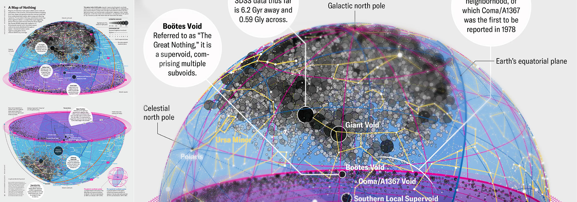
How Analyzing Cosmic Nothing Might Explain Everything
Huge empty areas of the universe called voids could help solve the greatest mysteries in the cosmos.
My graphic accompanying How Analyzing Cosmic Nothing Might Explain Everything in the January 2024 issue of Scientific American depicts the entire Universe in a two-page spread — full of nothing.

The graphic uses the latest data from SDSS 12 and is an update to my Superclusters and Voids poster.
Michael Lemonick (editor) explains on the graphic:
“Regions of relatively empty space called cosmic voids are everywhere in the universe, and scientists believe studying their size, shape and spread across the cosmos could help them understand dark matter, dark energy and other big mysteries.
To use voids in this way, astronomers must map these regions in detail—a project that is just beginning.
Shown here are voids discovered by the Sloan Digital Sky Survey (SDSS), along with a selection of 16 previously named voids. Scientists expect voids to be evenly distributed throughout space—the lack of voids in some regions on the globe simply reflects SDSS’s sky coverage.”
voids
Sofia Contarini, Alice Pisani, Nico Hamaus, Federico Marulli Lauro Moscardini & Marco Baldi (2023) Cosmological Constraints from the BOSS DR12 Void Size Function Astrophysical Journal 953:46.
Nico Hamaus, Alice Pisani, Jin-Ah Choi, Guilhem Lavaux, Benjamin D. Wandelt & Jochen Weller (2020) Journal of Cosmology and Astroparticle Physics 2020:023.
Sloan Digital Sky Survey Data Release 12
Alan MacRobert (Sky & Telescope), Paulina Rowicka/Martin Krzywinski (revisions & Microscopium)
Hoffleit & Warren Jr. (1991) The Bright Star Catalog, 5th Revised Edition (Preliminary Version).
H0 = 67.4 km/(Mpc·s), Ωm = 0.315, Ωv = 0.685. Planck collaboration Planck 2018 results. VI. Cosmological parameters (2018).
constellation figures
stars
cosmology
Error in predictor variables
It is the mark of an educated mind to rest satisfied with the degree of precision that the nature of the subject admits and not to seek exactness where only an approximation is possible. —Aristotle
In regression, the predictors are (typically) assumed to have known values that are measured without error.
Practically, however, predictors are often measured with error. This has a profound (but predictable) effect on the estimates of relationships among variables – the so-called “error in variables” problem.

Error in measuring the predictors is often ignored. In this column, we discuss when ignoring this error is harmless and when it can lead to large bias that can leads us to miss important effects.
Altman, N. & Krzywinski, M. (2024) Points of significance: Error in predictor variables. Nat. Methods 20.
Background reading
Altman, N. & Krzywinski, M. (2015) Points of significance: Simple linear regression. Nat. Methods 12:999–1000.
Lever, J., Krzywinski, M. & Altman, N. (2016) Points of significance: Logistic regression. Nat. Methods 13:541–542 (2016).
Das, K., Krzywinski, M. & Altman, N. (2019) Points of significance: Quantile regression. Nat. Methods 16:451–452.
Convolutional neural networks
Nature uses only the longest threads to weave her patterns, so that each small piece of her fabric reveals the organization of the entire tapestry. – Richard Feynman
Following up on our Neural network primer column, this month we explore a different kind of network architecture: a convolutional network.
The convolutional network replaces the hidden layer of a fully connected network (FCN) with one or more filters (a kind of neuron that looks at the input within a narrow window).
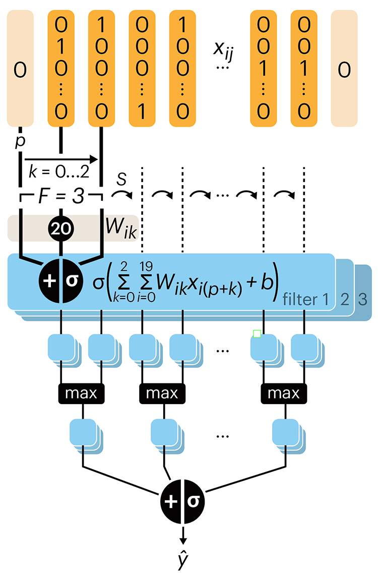
Even through convolutional networks have far fewer neurons that an FCN, they can perform substantially better for certain kinds of problems, such as sequence motif detection.
Derry, A., Krzywinski, M & Altman, N. (2023) Points of significance: Convolutional neural networks. Nature Methods 20:1269–1270.
Background reading
Derry, A., Krzywinski, M. & Altman, N. (2023) Points of significance: Neural network primer. Nature Methods 20:165–167.
Lever, J., Krzywinski, M. & Altman, N. (2016) Points of significance: Logistic regression. Nature Methods 13:541–542.