color summary statistics
- What is the purpose of the color summarizer?
- What good is this information?
- What color information is reported?
- How is average hue computed and reported?
- How are the histograms calculated?
- How are the color clusters computed and reported?
- How are color names determined?
output format
- What is the output format of the API?
- What is the format of the aggregate statistics lines?
- What is the format of the histogram lines??
- What is the format of the pixel lines?
- What is the format of the cluster lines?
describing color
color spaces and perceptual uniformity
- What is a color space?
- What does it mean for a color space to be perceptually uniform?
- How is the distance between two colors calculated?
- What are Brewer palettes, and why should I care?
color summary statistics
The color summarizer reports a summary of colors in an image using clustering, to group similar colors together and derive a set of colors that are representative of the image, histograms of color components (RGB, HSV, LCH, LAB), and descriptive statistics for components in each of the color space.
The name of the average color for each color cluster (or its closest named neighbor) is also provided, as is the set of words formed by the names of all neighbors within ΔE ≤ 5.
Using the color clusters, you can categorize and group images. For example, the hue from the cluster with the largest number of pixels can be inserted into the image's metadata to allow you to recall all images with a specific hue.
Another way to use clusters is to match the image to a suitable background. For example, you might use the rule that the background match the hue of the first cluster that has no more than half of the number of pixels than the next larger cluster. Using the hue, you could then adjust the lightness and chroma yourself to create a dark or light background, depending on whether the image itself is light or dark.
The summarizer was at one point used to annotate photos in the Flickr Color Fields group. These annotations permit users to search photos by its color characteristics.
The summarizer reports the average, median, minimum and maximum values for each components in RGB, HSV, Lab and LCH color models.
The format of this information is described below.
The average hue is calculated using mean of circular quantities. The standard way of computing the average cannot be used because hue is a periodic quantity (modulo 360).
Given a set of `N` hues `H=\{h_1, h_2, ...\}` in the range `h_i \in [0,359]`, first convert each hue to radians by using `h^r_i = \tfrac{\pi h_i}{180}` and then determine the angle formed by the average vector of all the hue angles. $$ \bar{h}^r = \arctan \left( \text{avg}_{i} \sin h^r_i, \text{avg}_{i} \cos h^r_i \right) $$
The `\bar{h}^r` is then converted to degress using `\tfrac{180}{\pi} \bar{h}^r \pmod {360}`.
The length of the average vector is also calculated using $$ \|\bar{h}\| = \sqrt { \left( \text{avg}_{i} \sin h^r_i \right)^2 + \left( \text{avg}_{i} \cos h^r_i \right)^2 } $$
Both `\bar{h}^r` and `\|\bar{h}\|` are reported. If all the hues in the image are similar, `\|\bar{h}\|` will be close to 1. If the image contains a balance of complementary hues, then `\|\bar{h}\|` will be close to 0.
The RGB, HSV, LCH and Lab components for each pixel are rounded to the nearest integer.
The ranges of each component are as follows.
- RGB `(R,G,B) \in [0-255]`
- HSV `H \in [0,359], (S,V) \in [0,100]`
- LCH `(L,C) \in [0,100], H \in [0,359]`
- Lab `L \in [0,100], (a,b) \in [-127,127]`
Colors in Lab space is calculated for all pixels and clustered using k-means clustering.
Briefly, k-means clustering partitions the pixels into k sets as to minimize the within-cluster sum of squares, calculated by the Euclidian distance to the center of the cluster, which is taken to be the average of the set.
The Lab space is used because it is perceptually uniform. The clustering requires that you specify the number of clusters ahead of time. You can select anywhere between 2 and 10 clusters.
For each cluster the following quantities are reported: fraction of image pixels in this cluster, average cluster color in RGB, HSV, LCH and Lab, the closest named color to the average cluster color and the words formed by all named colors within ΔE ≤ 5.
Output format is described here.
I curate a large list of named colors. As of 11 Jun 2016, this list has 8,332 colors. It is compiled from various sources, such as wikipedia, UNIX X11, raveling, resene and others.
Read about details here.
output format
The API provides aggregate statistics, color histograms, individual pixel values and color clusters. Each of these is reported on lines preceeded by the text stat, hist, pixel and cluster, respectively.
Below is the description of the plain-text output. XML and JSON output contains the same information, but in marked-up format.
When you are parsing the plain-text output, you should not assume a specific order to statistics or color spaces. The order is arbitrary, but reproducible. In other words, a line like
pix 1 0 cluster 1 hsv 208 46 63 lab 52 -4 -23 lch 52 23 259 rgb 87 127 161
will always have rgb as the last color space if you run the image again. However, if the code changes, the order might change as well.
When parsing these with a script, chop the string up into groups of 4 and identify the color space by its label (e.g. rgb), instead of assuming it.
Aggregate statistics are reported on lines labeled by stat.
The format of these lines is
stat COLOR_SPACE COMPONENT STATISTIC VALUE

 COLOR_SPACE : hsv    lab    lch    rgb
 COMPONENT   : h s v  l a b  l c h  r g b
 STATISTIC   : avg median min max
For example, here are the aggregate statistics for the LCH color space for an image
stat lch c avg 16
stat lch c median 19
stat lch c min 0
stat lch c max 26
stat lch h avg 253 1.00
stat lch h median 252
stat lch h min 0
stat lch h max 360
stat lch l avg 47
stat lch l median 53
stat lch l min 1
stat lch l max 84
The average hue value stat * h avg contains two values, as described above.
Histograms for each component of color spaces is reported in lines labeled by hist.
The format of these lines is
hist COLOR_SPACE COMPONENT VALUE NUM_PIXELS
For example,
hist lch c 0 5
hist lch c 1 100
hist lch c 2 127
...
hist lch c 24 97
hist lch c 25 17
hist lch c 26 7
hist lch h 0 2
hist lch h 2 2
hist lch h 3 2
...
hist lch h 350 3
hist lch h 354 2
hist lch h 360 4
hist lch l 1 5
hist lch l 2 93
hist lch l 3 59
..
hist lch l 82 12
hist lch l 83 17
hist lch l 84 6
where a line like
hist lch l 82 12
means that there were 12 pixels in the image with luminance `L = 82`.
Only values for which pixels in the image exist are shown—if there were no pixels with `L = 82` then this luminance value would not be listed in the histogram. This is why the maximum component value in each histogram is the maximum value in the image (e.g. `C = 26`) and not the maximum possible value in the color space.
Information about each pixel is reported in lines labeled by pixel.
The format of these lines is
pix X Y cluster CLUSTER_IDX { COLOR_SPACE COORDINATES }

 X : x position of pixel (0-indexed)
 Y : y position of pixel (0-indexed)
 CLUSTER_IDX : pixel cluster index, if clustering is on pixel has been assigned to a cluster (-1 otherwise)
 COLOR_SPACE : hsv    lab    lch    rgb
 COORDINATES : coordinates in the color space
For example,
pix 0 0 cluster 1 hsv 209 46 63 lab 51 -4 -23 lch 51 23 261 rgb 87 125 160
pix 1 0 cluster 1 hsv 208 46 63 lab 52 -4 -23 lch 52 23 259 rgb 87 127 161
pix 2 0 cluster 1 hsv 205 46 62 lab 52 -6 -21 lch 52 22 254 rgb 86 128 159
...
pix 38 8 cluster 2 hsv 204 38 71 lab 62 -7 -19 lch 62 20 250 rgb 113 154 182
pix 39 8 cluster 2 hsv 204 38 71 lab 61 -7 -19 lch 61 20 250 rgb 112 153 181
pix 40 8 cluster 1 hsv 205 39 71 lab 61 -7 -20 lch 61 21 251 rgb 111 153 182
pix 41 8 cluster 1 hsv 205 39 71 lab 61 -7 -20 lch 61 21 251 rgb 110 152 181
pix 42 8 cluster 2 hsv 204 39 71 lab 61 -7 -19 lch 61 20 250 rgb 110 152 180
pix 43 8 cluster 2 hsv 204 39 71 lab 61 -7 -19 lch 61 21 249 rgb 110 153 181
pix 44 8 cluster 1 hsv 205 40 71 lab 61 -7 -20 lch 61 21 252 rgb 110 152 182
pix 45 8 cluster 1 hsv 205 39 71 lab 61 -7 -20 lch 61 21 251 rgb 110 152 181
pix 46 8 cluster 2 hsv 204 39 71 lab 61 -7 -19 lch 61 20 250 rgb 110 152 180
pix 47 8 cluster 2 hsv 204 39 71 lab 61 -7 -19 lch 61 21 249 rgb 110 153 181
...
The cluster index is the same index as appears in the cluster lines, which are described below.
The color clusters are described by lines labeled by cluster.
The format of these lines is
cluster IDX n NUM_PIXELS f FRACTION_PIXELS { COLOR_SPACE COORDINATES }
        { NAMED_NEIGHBORS } NEAREST_NEIGHBORS NAMES_NEAREST_HEIGHBORS
For an example, let's look at this output
cluster 0 n 1171 f 0.312266666666667 rgb 58 84 108 hex #3A546C hsv 208 47 42 lab 35 -3 -17 lch 35 17 260 xyz 0.08 0.08 0.15 cmyk 20 9 0 58 fiord[6488][64,81,105](2.9):spinnaker[6337][47,77,102](2.9):wanaka[6317][40,73,98](5.0):dalek[6379][71,87,105](5.3):cello[6306][58,78,95](5.5):chathams_blue[6180][44,89,113](5.6):east_bay[6631][71,82,110](5.7):navigate[6130][48,78,94](5.7):spray_drift[6318][45,88,119](5.8):arapawa[6178][39,74,93](6.0) 3 fiord:spinnaker:wanaka

cluster 1 n 1122 f 0.2992 rgb 96 137 166 hex #6089A6 hsv 205 42 65 lab 55 -6 -20 lch 55 21 253 xyz 0.21 0.23 0.39 cmyk 28 12 0 35 air_force_blue[6226][93,138,168](1.4):rackley[6227][93,138,168](1.4):grey_blue[6264][107,139,164](3.2):hoki[6250][101,134,159](3.3):horizon[6153][90,135,160](3.4):greyish_blue[6291][94,129,157](3.6):bermuda_grey[6228][107,139,162](4.1):steel_blue[6308][90,125,154](4.5):slate_blue[6320][91,124,153](4.9):wedgewood[6225][78,127,158](5.0) 9 slate:air:bermuda:force:greyish:hoki:horizon:rackley:steel:blue:grey

cluster 2 n 886 f 0.236266666666667 rgb 127 161 184 hex #7FA1B8 hsv 205 31 72 lab 64 -6 -16 lch 64 17 249 xyz 0.3 0.33 0.5 cmyk 22 9 0 28 greyblue[6081][119,161,181](3.0):weldon_blue[6192][124,152,171](4.6):nepal[6230][142,171,193](4.7):blue_moon[6137][114,150,171](4.7):bluegrey[6082][133,163,178](4.8):bali_hai[6156][133,159,175](4.8):bluey_grey[6193][137,160,176](5.2):pewter_blue[6091][139,168,183](5.4):moonstone_blue[6088][115,169,194](5.6):grayish_azure[6323][125,147,168](5.8) 6 bali:bluegrey:greyblue:hai:moon:nepal:weldon:blue

cluster 3 n 392 f 0.104533333333333 rgb 20 25 28 hex #14191C hsv 199 29 11 lab 8 -2 -3 lch 8 3 236 xyz 0.01 0.01 0.01 cmyk 3 1 0 89 very_dark_azure[6349][17,23,29](2.6):bluish_black[6814][26,26,29](2.7):chimney_sweep[6508][28,29,31](3.1):charcoal[353][25,24,24](3.3):grey[7358][23,23,23](3.3):all_black[7359][24,24,24](3.3):grey[7360][26,26,26](3.3):cyanish_black[5744][26,29,29](3.3):eerie_black[7361][27,27,27](3.6):grey[7362][28,28,28](3.6) 10 dark:very:all:bluish:charcoal:chimney:cyanish:eerie:sweep:azure:black:grey

cluster 4 n 179 f 0.0477333333333333 rgb 207 187 181 hex #CFBBB5 hsv 14 13 81 lab 77 6 6 lch 77 8 43 xyz 0.52 0.52 0.51 cmyk 0 8 10 19 blanched_pink[1236][208,187,181](0.5):soulmate[1125][205,181,175](2.4):wafer[1436][212,187,177](2.6):cold_turkey[413][206,186,186](2.8):misty_rose[662][205,183,181](2.9):mistyrose[663][205,183,181](2.9):cold_turkey[808][202,181,178](3.0):dover_white[1434][201,191,187](4.1):quarter_imagine[1435][201,191,187](4.1):half_cloudy[2125][198,190,183](4.1) 10 misty:blanched:cloudy:cold:dover:half:imagine:mistyrose:quarter:soulmate:turkey:wafer:pink:rose:white
There are 5 clusters, indexed 0 to 5. The number of pixels in each cluster is 1171, 1122, 886, 392 and 179, respectively, and these compose 31%, 30%, 24%, 10% and 5% of the image.
The color of each cluster, formed from the average LCH coordinates of the colors assigned to the cluster, is reported next, in a variety of color spaces. For example, the first cluster has coordintes
rgb 58 84 108 hex #3A546C hsv 208 47 42 lab 35 -3 -17 lch 35 17 260 xyz 0.08 0.08 0.15 cmyk 20 9 0 58
For each cluster, the nearest neighbours from the large list of named colors is listed next. The neighbours appear as a list, delimited by : and neach neighbour has the format
NAME[IDX][RGB][deltaE]

 NAME   : name of color
 IDX    : index of color in the large list of named colors
 RGB    : RGB coordinates of color in the list
 deltaE : distance in LCH space from the named color to the cluster
For example, for the first cluster the nearest neighbours are
fiord[6488][64,81,105](2.9)
spinnaker[6337][47,77,102](2.9)
wanaka[6317][40,73,98](5.0)
dalek[6379][71,87,105](5.3)
cello[6306][58,78,95](5.5)
chathams_blue[6180][44,89,113](5.6)
east_bay[6631][71,82,110](5.7)
navigate[6130][48,78,94](5.7)
spray_drift[6318][45,88,119](5.8)
arapawa[6178][39,74,93](6.0)
where I've removed the : delimiter that joins these strings together. The index of the color in the named list is probably not going to be important to you, unless you want to make a lookup.
The final two fields is the number of nearest named neighbors within `\Delta E \le 5` and their names.
describing color
Each of these is a color space. A color space defines a subset of colors for which a set of numbers used to describe the color can be directly mapped to the manner in which the human eye responds to the color (trichromaticity values).
In contrast, a color model, which you may see used interchangebly with "color space" (sometimes correctly and sometimes not), is a mathematical recipe for expressing a color value using a set, usually three (e.g. RGB, HSV), of numbers.
See the answer to What is a color space? below for more details about the difference between color models and spaces.
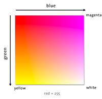
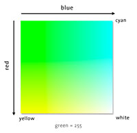
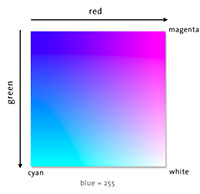
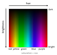
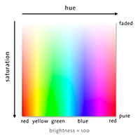
In each of RGB, HSV, HLS and HSI, hue is defined the same way and is generally taken to be in the range of 0-359 with hue = 0 being equivalent to hue = 360. Hue can be visualized as an angle. In the equation below the values of R, G, B are normalized to 1. $$ H = \arccos \frac{ \tfrac{1}{2}(2R-G-B)}{\sqrt{(R-G)^2-(R-B)(G-B)}} {\tag 1} $$
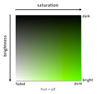
In HSV the saturation and value (the color summarizes uses this model) are calculated thus $$ S_{HSV} = \frac{\max (R,G,B) - \min (R,G,B)}{\max (R,G,B)} {\tag 2} $$ $$ V_{HSV} = \max(R,G,B) {\tag 3} $$
To complicate things a little bit, it is possible to define saturation without normalization, as `\max(R,G,B)-\min(R,G,B)`. In this definition, saturation is bounded by the value (brightness) of the color and corresponds to a conical color model (vs a cylindrical one in which saturation is normalized).
In HLS, lightness is calculated first because its value impacts how saturation is calculated. $$ L_{HLS} = \frac{\max(R,G,B)+\min(R,G,B)}{2} {\tag 4} $$ $$ S_{HLS} = \begin{cases} \frac{\max(R,G,B)-\min(R,G,B)}{\max(R,G,B)+\min(R,G,B)} & \text{if $L < 0.5$} \\[2ex] \frac{\max(R,G,B)-\min(R,G,B)}{2-\max(R,G,B)-\min(R,G,B)} & \text{if $L \ge 0.5$} {\tag 5} \end{cases} $$
Finally, in HSI (sometimes written as IHS) the intensity and saturation are given by $$ I_{HSI} = \frac{R+G+B}{3} {\tag 6} $$ $$ S_{HSI} = 1 - \frac{3\min(R,G,B)}{R+G+B} {\tag 7} $$
Although the scale for RGB, HSV and HLS varies from application to application, in general R, G, B are reported in the range 0-255, H in the range 0-359, and S, B, V and L are mapped onto the range 0-100.
Although hue is defined consistently, the definition of value/brightness, lightness and intensity are all different. Even though the terms sound similar, only two are synonyms.
Value and brightness are both defined as the maximum R,G,B component.
Lightness is the midpoint between the maximum and minimum R,G,B values.
Intensity is the average R,G,B value.
color spaces and perceptual uniformity
What is a color space
The difference between a model and a space is additional information needed to fully define the a space, such as characteristics of the primaries and viewing conditions. Another way to look at it is that you need a model to express quantitatively a color found in a color space, but you do not need the full machinery of a color space to make use of a color model.
For example, when RGB is interpreted as a color model, all it conveys is that an RGB color is denoted by three values, each being the amount of red, green and blue in the color. However, the model does not tell you what "red" is, nor how the eye reacts to it. It's common to have different kinds of "red", such as different red phosphors in different monitors.
RGB is an additive color space and each of the numbers represents the amount of red, green and blue components in a color. RGB is a device dependent color space meaning that a particular RGB value is a recipe given to a device, such as a monitor, to display a particular color. RGB is device dependent because any two monitors are unlikely to display the same color given an RGB triplet. The display on a monitor is dependent on a large number of factors: spectrum of phosophors and backlight, factory calibration, and user settings being some.
HSV is the hue/saturation/value color space. HSV is also known as HSB with "brightness" replacing "value". HLS is the hue/lightness/saturation color space. Finally HSI is the intensity/hue/saturation color space.
color space resources
The Wikipedia color space article is a great departure point for learning about color spaces. EasyRGB organizes the conversion equations between color spaces in one convenient list. Bruce Lindbloom's conversion table is also worth checking out. Bruce has a lot of interactive calculators on his site which are very helpful in getting your head wrapped around the variety of ways to describe color.
What does it mean for a color space to be perceptually uniform?
A color space is perceptually uniform if the mathematical distance (e.g. Euclidian, or otherwise defined by the metric of the space) between colors is prortional to the perceived difference between the colors.
One way in which this difference can be quantified is ΔE, as described below.
How is the distance between two colors calculated?
The ΔE is a measure of color difference distance between two colors in Lab space, `(L_1,a_1,b_1)` and `(L_2,a_2,b_2)` given by $$ \Delta E = \sqrt { (L_2-L_1)^2 + (a_2-a_1)^2 + (b_2-b_1)^2} $$
This is the Euclidian distance between the color points in the three-dimensional Lab space.
What are Brewer palettes, and why should I care?
I love Brewer palettes because they take the guess work out of color selection for figures and charts.
For more details, see my Brewer palette article.